
In Through the Looking Glass by Lewis Carroll, Alice and the White Queen had this exchange:
`I don't understand you,' said Alice. `It's dreadfully confusing!'
`That's the effect of living backwards,' the Queen said kindly: `it always makes one a little giddy at first--'
`Living backwards!' Alice repeated in great astonishment. `I never heard of such a thing!'
... `For instance, now,' she went on, ... `there's the King's Messenger. He's in prison now, being punished: and the trial doesn't even begin till next Wednesday: and of course the crime comes last of all.'
`Suppose he never commits the crime?' said Alice.
`That would be all the better, wouldn't it?' the Queen said ...
If there's to be a crime that comes last of all, it would be if you were to do poorly on the final exam. Although you are, like the King's Messenger, being punished now, it will be all the better if you never commit that crime. To that end your goal ought to be to learn calculus backwards and forwards, and I can tell you that up till now, you only know it forwards. So prepare to start learning it backwards, even though, as the White Queen observed, it might make you a little giddy at first.
In the last section we went to a lot of trouble to find the area under various functions using a method of slicing it into rectangles and taking the limit of the Riemann sum as the number of rectangles went to infinity. In each case, we came to a point where we had to find some clever trick that would evaluate a summation for us. And the tricks were different for different kinds of functions. Indeed it's pretty easy to imagine that for some functions that we might want to find the area under, the trick might be especially difficult. For example, I know of no trick for adding up
    n   ___
    å  Ök-1
   k=1
Yet that is precisely the summation you will be stuck with if you want to use the method from
the last section to find the area under the curve
             _
   f(x)  =  Öx
If we ever hope to find areas such as this, we need to find a better way of doing
them.
There is another trick you can use to find the area under the square root function, and it doesn't involve taking a Riemann sum of a bunch of square roots. Instead you can use what you already know from taking the limit of the Riemann sum of thef(x) = x2 function. Knowing what that area is can be the critical step to finding the area under the square root. First plot the square root function. Now pick a point on the curve and draw a horizontal line from that point to the y-axis. Draw a vertical line from that point to the x-axis. Note that you have described a rectangle. The curve divides the rectangle into two unequal areas. Turn the drawing on its side, and what do you see? When you have done your best to analyze this, click here.
| function | Area from x = 0 to x = a | |
| f(x) = mx | (1/2)ma2 | |
| f(x) = 3x + 4 | (3/2)a2 + 4a | |
| f(x) = x2 | (1/3)a3 | |
| f(x) = 2x | (1/ln(2))(2a - 1) | |
| f(x) = x1/2 | (2/3)a3/2 |
Observe that in every case, the table shows us that the area under the curve is a function of where the right-hand boundary, a, is of the region we wanted to find the area under. In fact I could replace each a with an x and call each of those area functions in the second column, F(x). Then the table would look like:
| Original function, f(x) | Area function, F(x) | |
| f(x) = mx | F(x) = (1/2)mx2 | |
| f(x) = 3x + 4 | F(x) = (3/2)x2 + 4x | |
| f(x) = x2 | F(x) = (1/3)x3 | |
| f(x) = 2x | F(x) = (1/ln(2))(2x - 1) | |
| f(x) = x1/2 | F(x) = (2/3)x3/2 |
I'd like you to try something now. Go down the list of F(x)'s in the second column of Table 10.2-2 and take the derivative of each one. That is, find F'(x) for each F(x) in the table. Try it.
There's something going on here that you can't miss even if you were dozing. In every case you should have found that
F'(x) = f(x)Perhaps it's an incredible coincidence, or perhaps I chose these examples in particular because they just happen to come out this way. Those two explanations sound implausible, eh? Indeed we have hit here on something that is so central to calculus that it is called The Fundamental Theorem of Calculus. And that is that finding one of these area functions is the opposite of finding a derivative. In other words, by finding the area function we have gone through the motions of finding a derivative, but we have done it backward. That is why, for every line of the table, the F(x) function is called an antiderivative of the f(x) function.
It also means that in order to find an area function for some f(x), you don't have to go through all the work of setting up the Riemann sum and taking the limit. You only have to find the function, F(x), whose derivative is your original function, f(x). Often this is easier said than done, but even when it's difficult, it's still easier than that nasty summation business we did in the last section.
Before we go ahead and prove this thing, let's try to put it into some real-world context. Suppose you have an object, say a train, that is in motion. You will recall that if x(t) is its position as a function of time, t, and v(t) is its velocity as a function of time, then
                      dx
   v(t)  =  x'(t)  =                                              eq. 10.2-1
                      dt
If v were constant, you would be able to find the position
of the train easily if you knew only where it started from, x0,
and what the time, t, was. You have the familiar motion equation that
you learned in algebra:
x = x0 + vt eq. 10.2-2But if the train's velocity is constant, say 30 miles per hour, how are the passengers ever going to get on or off the train? So to add some realism to the situation, let's suppose that starting at the moment the train begins pulling out of the station, its velocity is given by
v(t) = at eq. 10.2-3where a is a constant acceleration. Now how do we find the train's position as a function of time? Clearly from equation 10.2-1, x(t) must be an antiderivative of v(t). But look at what's going on in more detail.
At time,
x11 = x10 + (1 second × v) = x10 + (1 second × 10a) eq. 10.2-4Next we allow that at the moment of
x12 = x11 + (1 second × 11a) eq. 10.2-5If you imagine holding the velocity constant throughout each second and doing the sum for each second the train travels, the equation for the kth second is
xk = xk-1 + (1 second × (k-1)a) eq. 10.2-6Can you see that what you really end up with is a Riemann sum? The equation is saying that this x is the sum of something plus the last x. Of course that last x was the sum of something plus the x before that, and so on. So really, this x is the sum of all those somethings, going back to the very first x. So this x is the sum:
                  n
   xn  =  x0  +   å 1 second × (k-1)a                            eq. 10.2-7
                 k=1
where n is the number of seconds elapsed since the train left
the station.
Of course the train's velocity is not constant, even over the period of just a second. So our assumption that it is will lead to some inaccuracy in the approximation, xn, of the train's position after n seconds. But you will agree that trains' velocities don't change a whole lot in the span of a second. And if this method leads to too much inaccuracy, you could always do it by a shorter interval instead -- say by the millisecond. Since there are a thousand milliseconds in each second, you will have to sum a thousand times more terms, but that's the price you pay for accuracy, right? Of course you could take the limit as the short interval of time goes to zero and the number of intervals goes to infinity. That should give you a perfect approximation of position as a function of time. But isn't that exactly what we were doing in the last section?
The point is, we know that position as a function of time is an antiderivative of velocity. And we know that we can also get position from velocity by taking the limit of a Rieman sum. This suggests that the limit of the Riemann sum of velocity is always an antiderivative of velocity. Which is the thrust of the Fundamental Theorem of Calculus.
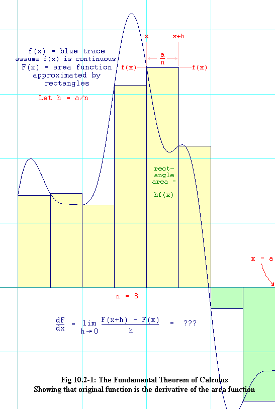
The figure shows an arbitrary function. It has already been divided into rectangles according to a left Riemann sum. Note that the last two rectangles on the right are of negative height. So their area is also considered negative, and that is shown by shading them green instead of yellow. The area function, F(x), is the area bounded from above by f(x), from below by the x-axis, from the left by the y-axis, and from the right by x. We know the area function, F(x), is the limit of the sum of the areas of the rectangles between zero and x as n goes to infinity.
Here is the key to understanding the Fundamental Theorem of calculus. Look at the fifth rectangle. In the diagram, we have chosen x to be its left-hand edge. Its height is f(x). Its width is a/n, which we have chosen to call h. So the area of that rectangle is hf(x). Observe that as n goes to infinity, h will go to zero.
The area function of the x we have chosen (that is F(x) at the left edge of the fifth rectangle) is approximated by the sum of the areas of the first four rectangles. The area function of x+h (that is F(x+h), which is at the right edge of the fifth rectangle) is approximated by the sum of the first five rectangles. So the difference between F(x+h) and F(x) must be approximated by the area of the fifth rectangle. And that area is shown on the diagram to be equal to hf(x). Read this paragraph over if you don't get it at first. And look carefully at the diagram.
The result of this observation is the following
F(x+h) - F(x) » hf(x) eq. 10.2-8
| You might be thinking, "But when you make the rectangles smaller and smaller, x is no longer the left-hand edge of the fifth rectangle. So how can this proof still work?" No problem. Remember that to make h go to zero, we have to have n going to infinity. But there is no restriction on how it goes to infinity. In figure 10.2-1, we could start out by doubling n. Now our x as at the left edge of the tenth rectangle (we never said there was anything special about the fifth rectangle except that x is at its left edge for the n shown in the figure). This rectangle is only half as thick as the fifth one was before we doubled n. Next choose triple the original n, and the rectangle will be only one third as thick. The x will be the left edge of the fifteenth rectangle now. Then use quadruple the original n with x at the left edge of the twentieth rectangle, and so on. n goes to infinity, h goes to zero, x remains the same, and everything is ok. |
Look again at the diagram. If you hold the left-hand edge of the rectangle fixed and allow the right-hand edge to get closer and closer to it, can you see how the area of the skinnier and skinnier rectangle becomes a better and better approximation of the area under that slice of the curve?
So what is the derivative of F(x)? We use the limit formula for derivatives to find that:
                    F(x+h) - F(x)
   F'(x)  =   lim                                                 eq. 10.2-9a
             h  > 0       h
But in the limit, we know we can replace
                    h f(x)
   F'(x)  =   lim                                                 eq. 10.2-9b
             h  > 0    h
This limit is a snap.
F'(x) = f(x) eq. 10.2-9cAnd that is the proof of the Fundamental Theorem of Calculus. That is it shows that the area function is always an antiderivative of the original function. Of course we have relied on the fact that the Riemann sum always has a limit as n goes to infinity, which we have not bothered to prove here. A discussion of how to prove this is optional material that you can view by clicking here.
Suppose three trains accelerate away from the station, again at
a rate of
Clearly they are never in the same position at the same time. And that means that they all have different position functions. Yet all three of these position functions are antiderivatives of the same velocity function. How can this be?
| Position Function | Velocity Function | |
| x1(t) = (1/2)at2 + D | v1(t) = at | |
| x2(t) = (1/2)at2 + K | v2(t) = at | |
| x3(t) = (1/2)at2 + C | v3(t) = at |
Perhaps you have noticed in the text so far that I have never referred to the antiderivative of a function, only to an antiderivative of a function. Now you will come to understand why.
The positions of Denver, Kansas City, and Cincinnati are all constants. After all, the cities don't move. Call their positions D, K, and C respectively. The table shows the position function of each of the trains in the left-hand column. If you take the derivative of each of those position functions with respect to t, you see that each time you get the velocity function, v(t), and they are all exactly the same.
What's happening here is something that you already knew about. And that is that
the derivative of a constant is always zero. This means that if you
have a function, f(x), and you go and find its antiderivative,
F(x), then you can always come up with other antiderivatives
of f(x) simply by adding constants to F(x).
So
 |
 |
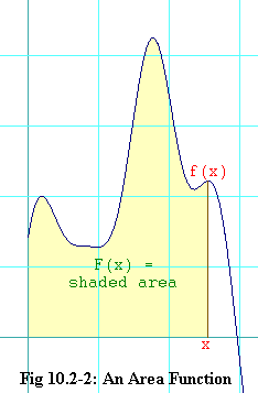
Now think back to the area functions we talked about earlier. To find the area function, F(x), we always used the area bounded on the left by the y-axis and on the right by x, as shown in the figure 10.2-2. We use x as one of the vertical boundaries because it is the independent variable of the area function, F(x). But what is so special about the y-axis that we must always use it as the other vertical boundary? Nothing at all.
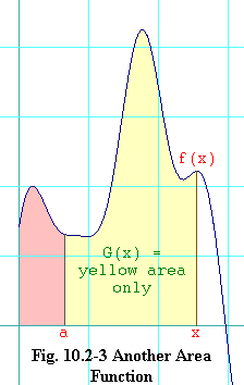
Figure 10.2-3 shows the same f(x), but a different area function. Instead of using the y-axis as the left-hand boundary, we use the vertical line at a, where a is held constant. G(x) is the yellow area in this diagram. Like F(x), this new area function varies as we move x right or left. The difference between F(x) and G(x) is the pink area. Since a is a constant, the pink area is constant as well. In other words, F(x) and G(x) differ by a constant.
What about the derivatives of F(x) and G(x)? Since both are area functions of f(x), the Fundamental Theorem of Calculus applies. So it must be that
F'(x) = G'(x) = f(x) eq. 10.2-10What this means is that it doesn't matter where you take the left-hand vertical boundary to be, as long as you take it to be constant. The resulting area function is still an antiderivative of the original function.
Suppose you had
                      1
   F'(x)  =  f(x)  =                                              eq. 10.2-11
                      x
If we choose F(1) = ln(1) + C = 0 eq. 10.2-12
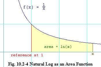
Since
Finding the constant, C, that makes an antiderivative work for
some special set of circumstances is called solving a boundary condition.
In the example we just did, we found a general antiderivative based upon our
existing knowledge of what the derivative of the ln(x) function is.
That antiderivative had an unknown constant, C, in it.
Then we solved the
boundary condition of
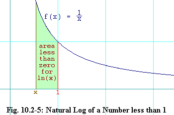
What if we use the same definition for the area function, but this time instead
of choosing an x greater than 1, we choose
| x is left of reference | x is right of reference | |
| f(x) is negative | ||
| f(x) is positive |
Table 10.2-4 shows how to determine the sign (or polarity) of an area that you get from an area function. You need to know which direction (right or left) you are taking the area in, and whether your f(x) is positive or negative over the region you are taking the area of.
If you find the table confusing, remember the train. In our discussion of the train a little while back, we figured out the distance the train had traveled after it left the station. But how about where it was before it got to the station. Think of the time it was at the station as the reference point. If the train was always moving east (i.e. moving in the positive direction, which we shall say is east) then before it got to the station, it was west of the station (negative area) and afterward it was east of the station (positive area). But if the train was going west (i.e. moving in the negative direction), then it was east of the station (positive area) before getting to the station and west of the station (negative area) afterward.
Section 10.3: Grist for the Mill -- Definite and Indefinite Integrals Still under construction