Exploring the Input Bar

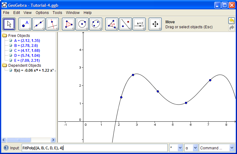
Open a new GeoGebra worksheet.   I have selected Options > Labeling > No New Objects. Place 5 points randomly.  We'll find the polynomial of degree 4 that best fits these points. At the bottom right corner of your screen is the Command List.  Open it up to see what commands are available to you.  Select FitPoly.  Type the F1 key to see what form its argument takes.  You should see   FitPoly[<list of points>, <degree of polynomial>] Lists are sets of objects delimited by braces { }.  Type   FitPoly[ { A, B, C, D, E }, 4 ] Now move the points and see what happens.  Type  Integral[f(x), 2, 6]  to see its effects. Click the (?) icon to the left of the Input Bar for more information.
GeoGebra has some nice random number generation features. Enter P = (RandomBetween[1, 7], RandomBetween[1, 4] ) This generates a point with x-coordinate between 1 and 7 (inclusive) and y-coordinate between 1 and 4 (inclusive). Typing Ctrl-R (View > Recompute All Objects) will regenerate the random numbers.
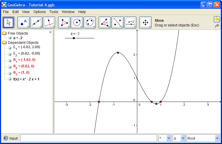
Create a slider named  a  and allow it to take values from -5 to 5. Define  f(x) = x^3 + a x Move the slider so a = -2. Type     R = Root[ f(x) ]    and     E = Extremum[ f(x) ] See how GeoGebra creates multiple points and names. See how these values change as the slider is moved.
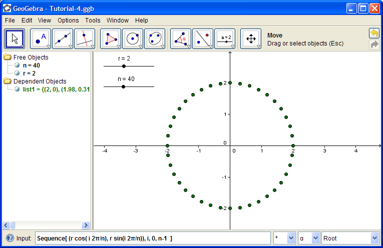
One of the most powerful commands is Sequence. Make a slider called  r  with values from 0 to 5. Make a slider called  n  with values from 1 to 100, incrementing by 1. Enter the command Sequence[ (r cos( i 2π/n), r sin(i 2π/n)), i, 0, n-1 ] To enter the π symbol, type Alt-p.  Be careful with parentheses. This creates a sequence of points (the first argument in the command) as  i  goes from 0 to n-1. Just for fun, right-click slider  r  and check Animation On.  Notice how a little Play/Pause button appears in the lower left corner of the Graphics View.

• Commands (like FitPoly) are capitalized and take their arguments inside brackets [ ], whereas built-in functions (like sin) are lowercase and take their arguments inside parentheses ( ).  You can find a list of built-in functions here.
• I often use the FitPoly feature to make polynomial graphs with certain features (max, min, etc.).  Then I copy the images for use in class presentations/quizzes/tests.
• The Sequence command creates a list of objects.  GeoGebra often uses lists of objects to do things.  A list is delimited by braces, for example, { 1, 2, 10, 2.3 }  or  { (0,1), (9,3), (7,6) }  or  {A, B, C}.  More on lists here.
  
• It's easy to use Greek letters for variables.  Type Alt-a for alpha, Alt-b for beta, etc.  You can see the list here.  However, π always represents the constant.