Definition. A vector is an ordered list of numbers \( (a_1, a_2, \ldots, a_n) \). We typically represent a vector as a column vector, which is a matrix with a single column: \[ \begin{bmatrix} a_1 \\ a_2 \\ \vdots \\ a_n \end{bmatrix} \] The numbers in the vector are called the "components" or "entries" of the vector.
We write \( \mathbb R^n \) for the set of all vectors with \( n \) entries. For now, we will focus on \( \mathbb R^2 \), but the basic operations we will discuss can be extended to any number of dimensions.
In these lecture notes and in any other printed format, we will typically use bold-faced, lower-case letters for vectors: \( \boldsymbol u, \boldsymbol v, \boldsymbol w \), and so on. In our handwriting, trying to make letters "bold-faced" is impractical, so instead we use a "vector hat" for vectors: \( \vec{u}, \vec{v}, \vec{w} \), and so on. These notations are used to distinguish vectors from "scalars" (also known as "numbers").
We can add two vectors: \[ \vectwo {-1} 2 + \vectwo 5 0 + \vectwo {-1+5} {2+0} = \vectwo 4 2 \]
We can also multiply a vector by a scalar: \[ 3 \vectwo {-1} 2 = \vectwo {3(-1)} {3(2)} = \vectwo {-3} 6 \]
Dividing a vector by a scalar is possible, but it is usually more convenient to think of that as multiplying the vector by a fraction: \[ \vectwo {-3} 8 \div 4 = \frac 1 4 \vectwo {-3} 8 = \vectwo {-3/4} 2 \]
It is important to understand the distinction between points and vectors: we can perform operations on vectors but not on points. One thing that we cannot do (yet) is multiply one vector by another.
Definition. If \( \bbm u = \vectwo {u_1} {u_2} \), \( \bbm v = \vectwo {v_1} {v_2} \), and \( c \) is a scalar, then \[ \bbm u + \bbm v = \vectwo {u_1} {u_2} + \vectwo {v_1} {v_2} = \vectwo {u_1 + u_2} {v_1 + v_2} \quad \mbox{and} \quad c \bbm u = c \vectwo {u_1} {u_2} = \vectwo {c\ u_1} {c\ u_2} \] We say that vector addition and scalar multiplication are performed "component-wise" since the operations happen independently in each component.
Definition. The zero vector, written \( \bbm 0 \) or \( \vec{0} \), is the vector whose entries are all zero. In \( \mathbb R^2 \), the zero vector is \( \bbm 0 = \vectwo 0 0 \).
The zero vector has some nice algebraic properties:
Typically, we will visualize a vector \( \vectwo a b \) as an arrow pointing from the origin \( (0,0) \) to the point \( (a,b) \). The originating point of a vector arrow is its "tail," and the ending point is its "head." The same vector can be drawn in any position, as long as its length and direction are preserved. When the tail of a vector is at \( (0,0) \), we say that the vector is in "standard position."
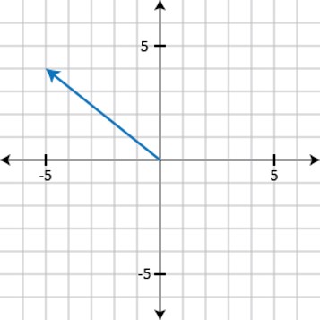
For example, consider the vector \( \bbm v = \vectwo {-5} 4 \). We can visualize this vector as an arrow from \( (0,0) \) to \( (-5,4) \):
This same vector could also have been represented by an arrow from \( (3,2) \) to \( (-2,6) \) since that arrow has the same length and direction.
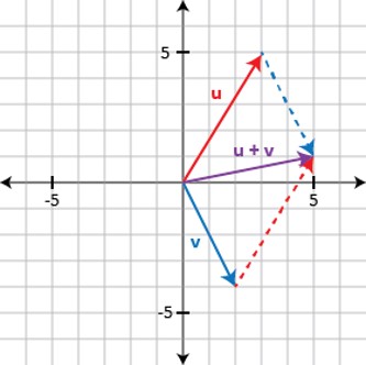
We can visualize the rule for adding vectors by using a parallelogram. Given vectors \( \bbm u \) and \( \bbm v \), place both vectors in standard position and then draw a parallelogram that has \( \bbm u \) and \( \bbm v \) as two of its sides. The diagonal of this parallelogram that points from the origin to the opposite corner is \( \bbm u + \bbm v \):
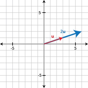
Scalar multiplication can be visualized as stretching or shrinking a vector. For example, multiplying a vector by 2 doubles its length and preserves the direction:
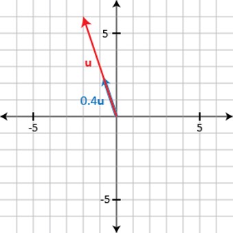
Multiplying a vector by 0.4 creates a vector that is 40% as long:
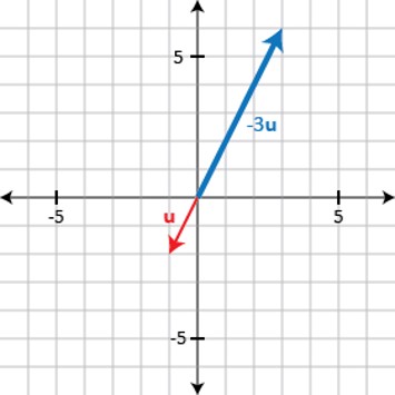
Multiplying a vector by a negative scalar stretches or shrinks the vector and also reverses its direction:
The definitions of vector addition and scalar multiplication can be extended to higher dimensions. To add two vectors in \( \mathbb R^n \), add the corresponding entries. To multiply a vector in \( \mathbb R^n \) by a scalar, multiply each entry by that scalar. The visualizations we discussed extend to \( \mathbb R^3 \), but things are harder to visualize in four or more dimensions.
The two vector operations we have discussed (vector addition and scalar multiplication) have several "nice" algebraic properties, as shown in the table below. The table also lists the names of these properties, some of which you may have seen before. These properties mean that we can use our "algebraic intuition" when working with these operations. It's important to emphasize that some of the operations that we will discuss later in this course don't follow all of our algebraic intuitions!
For all \( \bbm u, \bbm v, \bbm w \in \mathbb R^n \) and all scalars \( c\) and \( d \),
| (i) | \( \bbm u + \bbm v = \bbm v + \bbm u\) | Commutativity of Vector Addition |
| (ii) | \( (\bbm u + \bbm v) + \bbm w = \bbm u + (\bbm v + \bbm w) \) | Associativity of Vector Addition |
| (iii) | \( \bbm u + \bbm 0 = \bbm 0 + \bbm u = \bbm u \) | Additive Identity |
| (iv) | \( \bbm u + (-\bbm u) = (-\bbm u) + \bbm u = \bbm 0\), where "\( -\bbm u \)" denotes \( (-1)\bbm u \) | Additive Inverses |
| (v) | \( c(\bbm u + \bbm v) = c\,\bbm u + c\,\bbm v \) | Distributivity |
| (vi) | \( (c+d)\bbm u = c\,\bbm u + d\,\bbm u \) | Distributivity |
| (vii) | \( (cd)\bbm u = c(d\, \bbm u) \) | Compatibility |
| (viii) | \( 1\,\bbm u = \bbm u \) | Scalar Multiplication Identity |