In the previous lecture, we learned about a basis for a subspace, which is a linearly independent set of vectors that spans the subspace. One reason why bases are important is that they allow us to uniquely describe any vector in that subspace using coordinates.
Theorem (Uniqueness of Coordinates). Let \( H \) be a subspace of \( \mathbb R^n \), let \( \cal B = \{ \bbm b_1, \ldots, \bbm b_p \} \) be a basis for \( H \), and let \( \bbm x \in H \). There exist unique scalars \( c_1, \ldots, c_p \) for which \( \bbm x = c_1 \bbm b_1 + \cdots c_p \bbm b_p \).
We call these unique scalars the coordinates of \( \bbm x \) relative to the basis \( \cal B \) and write \( [\bbm x]_{\cal B} = \vecfour {c_1} {c_2} \vdots {c_p} \).
Proof of the Uniqueness of Coordinates Theorem. Since \( \cal B \) spans \( H \), there exists at least one set of scalars \( c_1, \ldots, c_p \) for which \( \bbm x = c_1 \bbm b_1 + \cdots c_p \bbm b_p \). Suppose that there also exists a set of scalars \( d_1, \ldots, d_p \) for which \( \bbm x = d_1 \bbm b_1 + \cdots d_p \bbm b_p \). Subtracting these two equations gives \[ \begin{eqnarray*} \bbm x - \bbm x & = & (c_1 \bbm b_1 + \cdots c_p \bbm b_p) - (d_1 \bbm b_1 + \cdots d_p \bbm b_p) \\ \bbm 0 & = & (c_1-d_1) \bbm b_1 + \cdots + (c_p-d_p) \bbm b_p. \end{eqnarray*} \]
Since \( \cal B \) is a linearly independent set, we have \( c_1 - d_1 = 0, \ldots, c_p - d_p = 0\). Thus, \( c_i = d_i \) for all \( i \), which proves that the scalars are unique. \( \Box \)
Example 1. Let \( \bbm v_1 = \vecthree 1 {-2} 3 \) and \( \bbm v_2 = \vecthree {-1} 0 {-4} \), and let \( H = {\rm Span}\{ \bbm v_1, \bbm v_2 \} \). Note that \( {\cal B} = \{ \bbm v_1, \bbm v_2 \} \) is a basis for \( H \). Let \( \bbm u = \vecthree 5 {-4} {18} \). Find \( [\bbm u]_{\cal B}\).
Note that the problem tells us that \( \cal B \) is a basis for \( H \), so we don't need to verify that ourselves. We only need to find scalars \( x_1 \) and \( x_2 \) for which \( x_1 \bbm v_1 + x_2 \bbm v_2 = \bbm u \). We set up and row-reduce the corresponding augmented matrix: \[ \begin{bmatrix} 1 & -1 & 5 \\ -2 & 0 & -4 \\ 3 & -4 & 18 \end{bmatrix} \longrightarrow \begin{bmatrix} 1 & 0 & 2 \\ 0 & 1 & -3 \\ 0 & 0 & 0 \end{bmatrix} \]
From this, we can see that the solution is \( x_1 = 2 \) and \( x_2 = -3 \). So, \( [\bbm u]_{\cal B} = \vectwo 2 {-3} \). \(\Box \)
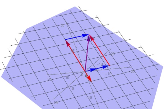
Note that, in Example 1, the vectors in \( H \) (including \( \bbm u \)) are in \( \mathbb R^3 \), but \( [\bbm u]_{\cal B} \) is a vector in \( \mathbb R^2 \). This is because the given basis for \( H \) has only two vectors. We can think of \( H \) as a rotated version of the \( xy \)-plane:
This image shows the subspace \( H \) and the vector \( \bbm u \), in purple, written as a linear combination of the basis vectors in \( \cal B \). The correspondence \( \bbm x \leftrightarrow [\bbm x]_{\cal B} \) is a linear transformation that is one-to-one and onto. We call such a transformation an isomorphism, and the study of isomorphisms is central to linear algebra and abstract algebra.
Theorem (Coordinate Isomorphism). Let \( H \) be a subspace of \( \mathbb R^n \) and let \( {\cal B} = \{ \bbm b_1, \ldots, \bbm b_p \} \) be a basis for \( H \). Let \( T : H \to \mathbb R^p \) be defined by \( T(\bbm x) = [\bbm x]_{\cal B} \). Then \( T \) is a linear transformation that is one-to-one and onto.
Proof. Let \( M \) be the matrix whose columns are \( \bbm b_1, \ldots, \bbm b_p \). By definition of coordinates, if \( \bbm x \in H \), then \( \bbm x = M[\bbm x]_{\cal B} \). The transformation \( S: \mathbb R^p \to H \) defined by \( S(\bbm x) = M\bbm x \) is a matrix transformation and is therefore linear. Since \( S \) and \( T \) are inverses, this proves that \( T \) is linear and also that \( T \) is one-to-one and onto. \( \Box \)
Example 2. Let \( \bbm u_1 = \vecthree 1 {-3} 2, \bbm u_2=\vecthree 2 1 {-4}\), and \(\bbm u_3 = \vecthree {-3} {-1} 0 \).
For (a), we can do this by row-reducing the matrix that has \( \bbm u_1, \bbm u_2, \bbm u_3 \) as its columns: \[ \begin{bmatrix} 1 & 2 & -3 \\ -3 & 1 & -1 \\ 2 & -4 & 0 \end{bmatrix} \longrightarrow \begin{bmatrix} 1 & 0 & 0 \\ 0 & 1 & 0 \\ 0 & 0 & 1 \end{bmatrix} \] Since this matrix has a pivot in every row and every column, \( \{ \bbm u_1, \bbm u_2, \bbm u_3 \} \) is linearly independent and spans \( \mathbb R^3 \).
For (b), we need to solve the equation \( x_1 \bbm u_1 + x_2 \bbm u_2 + x_3 \bbm u_3 = \bbm w \). We row-reduce the corresponding augmented matrix: \[ \begin{bmatrix} 1 & 2 & -3 & -4 \\ -3 & 1 & -1 & -2 \\ 2 & -4 & 0 & 1 \end{bmatrix} \longrightarrow \begin{bmatrix} 1 & 0 & 0 & 7/38 \\ 0 & 1 & 0 & -3/19 \\ 0 & 0 & 1 & 49/38 \end{bmatrix} \] So, \( [\bbm w]_{\cal B} = \vecthree {7/38} {-3/19} {49/38} \). \( \Box \)
Example 3. Let \( \bbm t_1 = \vecfour 0 {-1} {-2} 1 \), \(\bbm t_2 = \vecfour {-4} 1 0 {-1} \), and \( \bbm t_3 = \vecfour {-2} {-2} 1 0 \), and let \( H = {\rm Span} \{ \bbm t_1, \bbm t_2, \bbm t_3 \} \).
For (a), we already know that \( \cal B \) spans \( H \), so we only need to prove that \( \{ \bbm t_1, \bbm t_2, \bbm t_3 \} \) is a linearly independent set. We row-reduce the matrix that has these vectors as its columns: \[ \begin{bmatrix} 0 & -4 & -2 \\ -1 & 1 & -2 \\ -2 & 0 & 1 \\ 1 & -1 & 0 \end{bmatrix} \longrightarrow \begin{bmatrix} 1 & 0 & 0 \\ 0 & 1 & 0 \\ 0 & 0 & 1 \\ 0 & 0 & 0 \end{bmatrix} \] By the Linearly Independent Columns Theorem, since this matrix has a pivot in every column, its columns are linearly independent. Thus \( \cal B \) is a basis for \( H \).
We solve the equation \( x_1 \bbm t_1 + x_2 \bbm t_2 + x_3 \bbm t_3 = \bbm y \): \[ \begin{bmatrix} 0 & -4 & -2 & 0 \\ -1 & 1 & -2 & -4 \\ -2 & 0 & 1 & -2 \\ 1 & -1 & 0 & 2 \end{bmatrix} \longrightarrow \begin{bmatrix} 1 & 0 & 0 & 3/2 \\ 0 & 1 & 0 & -1/2 \\ 0 & 0 & 1 & 1 \\ 0 & 0 & 0 & 0 \end{bmatrix} \] This tells us that \( [\bbm y]_{\cal B} = \vecthree {3/2} {-1/2} 1 \). \( \Box \)
Note that, in Example 3b, we did not know in advance that \( \bbm y \in H \) before trying to find \( [\bbm y]_{\cal B} \). If it had turned out that \( \bbm y \notin H\), then we would have gotten a pivot in the last column of our augmented matrix, showing that the equation we were trying to solve had no solutions. Only vectors that are actually in the subspace have coordinates!
« Lecture 30 Back to Top Lecture 32 »