Section 10: Integrals

This section is still under construction

10.3 Grist for the Mill -- Definite and Indefinite Integrals

Return with me to the days of yore when, if the local miller didn't grind enough grain into flour, the whole community would go hungry. In the village I am picturing, there is but one mill. A dam holds back a brook to form a millpond. The water from the pond turns a waterwheel, which turns the mill, which grinds the grain. The demand for flour is so great that the miller and his sons work shifts to keep the mill productive twenty-four hours a day. So what limits production is how fast the pond water can turn the waterwheel. And that rate is in direct proportion to how high the water level is in the pond.

The miller needs to project his inventory far into the future in order to serve his customers well. To do this, he needs to know how much production he can get in any period. That period might be any week, any month, any quarter, or an entire year.

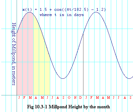
The problem is, the pond's water level varies seasonally. Based upon past weather patterns, the miller has determined that the water level that the water level, in meters, is

   x(t)  =  1.5  +  cos( (pt/182.5) - 1.2)                        eq. 10.3-1

where t is days past January first. Until now the miller's method of calculating production for any period has been to plot the water level as a function of time throughout that period on finely ruled graph paper. Then he simply counts the number of squares under the graph. He multiplies that by a conversion constant and out comes his production.

But counting all those tiny little squares on the graph paper got to be a strain on the old man's eyes, not to mention his patience. One evening his eldest son, who was learning calculus in his time off from the mill, saw his dad sweating over next quarter's projections.

"What you doin', Dad?" he asked. "Drat!" the miller exclaimed. "You've made me lose count." "Count of what?" So the miller explained the procedure to his son. "Why don't you just use antiderivatives?" the son asked. It was clear from the expression on the old man's face that it was the son's turn to explain things now. "Ok Dad. The fundamental theorem of calculus tells us that if you pick an antiderivative of your `x(t)` function it will be some area function of that same `x(t)`. It might not be the exact area function you are interested in, but it's easy to make it into the one you're interested in."
	Pink area is proportional to production for the January through March quarter.
	Yellow area is proportional to production for the April through June quarter.

"And how do you do that?" asked the dad.

"Look here. I can tell, because I know my derivatives, that an antiderivative of your x(t) = 1.5 + cos((pt/182.5) - 1.2) is

   X(t)  =  1.5t  +  (182.5/p)sin((pt/182.5) - 1.2)  +  C         eq. 10.3-2

where C is some undetermined constant. You can see that if you take the derivative of this X(t) you get your x(t). "

"Well that's just great," the dad complained. "I'll go and tell the village elders and the mortgage company that production numbers for next quarter are subject to an undetermined constant."

But Dad, it doesn't matter what C is. An antiderivative gives you the area under your curve from some fixed time past until a time of your choosing. Let's say that we chose C so that it gave it to us from the first of the year. You are trying to figure numbers for the second quarter. Now watch. I'll color the first quarter area on your graph pink and the second quarter area yellow. If I take X(t) for t at the end of the first quarter, it will give me the pink area. If I take it for t at the end of the second quarter it will give me the pink area plus the yellow area. So to get the yellow area, I merely subtract the first number from the second. So the first quarter ends at the end of the 90th day of the year. The second quarter ends at the end of the 181st day of the year. So the yellow area must be

   A_yellow  =  X(181) - X(90)

It's that easy."

"So what happened to the undetermined constant," asked the dad.

"Well just substitute in the expression for X(t) and you'll see.

   A_yellow  =  (1.5 × 181)  +  (182.5/p)sin((181p/182.5) - 1.2)  +  C

      -  (1.5 × 90)   -  (182.5/p)sin((90p/182.5) - 1.2)   -  C

The C cancels out exactly. So you don't have to care what it is. It will always cancel."

"But what if the pink area doesn't start at the beginning of the year? What about that, Mr. Too-Much-Education?"

"It still doesn't matter. You're just asking what would happen if the pink area started at a different time. But you will always be taking the pink plus the yellow and subtracting away the pink. The pink always cancels no matter where it starts. The difference will always give you the yellow area. Whatever your yellow area is, just take an antiderivative at the t where it ends and subtract that same antiderivative at the t where it begins. All you need to do is plug your choice of antiderivative function into your pocket calculator and you've got the production projections."

"Just one problem," said the dad. "We're living in the days of yore. Pocket calculators won't be invented for another 300 years."

The function, X(t), shown in equation 10.3-2 is called the indefinite integral of the x(t) shown in equation 10.3-1. The notation the world uses to represent this is

1.5 + cos((pt/182.5) - 1.2) dt =

1.5t + (182.5/p)sin((pt/182.5) - 1.2) + C eq. 10.3-3

The funny squiggly symbol is called an integral sign. The equation is saying that the expression to the right of the equal is an antiderivative of everything between the integral sign and the dt. The dt tells us that we are taking the antiderivative with respect to the independent variable, t. So if you take the derivative of the function to the right of the equal with respect to t, you should get the function that lies between the integral sign and the dt. The function between the integral sign and the dt is called the integrand. The function to the right of the equal is called the indefinite integral of the integrand. We say it's indefinite because it contains that undetermined constant, C.

But if we do as the miller's son suggested and evaluate the indefinite integral at both t = 90 and at t = 181, and then take the difference, we get a thing we call a definite integral.

181 90

1.5 + cos((pt/182.5) - 1.2) dt = 171.2889333 meter-days eq. 10.3-4

The numbers at the top and bottom of the integral sign are called limits of integration. We say we are taking the definite integral of this integrand from 90 to 181. And if those limits are constants, as they are here, what we get out is not a function but a number. The value, 171.2889333 meter-days, is what the miller was after when he was counting the tiny squares on his graph paper.

Observe the units of the answer. The units of the integrand function is meters, because it is measuring how high the water in the millpond is. The units of the span over which we took the definite integral is days, which is also the units of the dt operator. The units of the definite integral will always be the product of the units of the integrand with the units of the independent variable. So here we get meters times days. You will notice that that is also the units of area on our graph (figure 10.3-1) -- that is the horizontal axis is in days, the vertical axis is in meters, so any rectangle in that graph has area with units of meters times days.

You can always distinguish between a definite integral and an indefinite integral because only the definite integral has limits above and below the integral sign.

The procedure for evaluating a definite integral is

Find the indefinite integral first. This is not always easy, and we will discuss how to do it in the next section.
Since the undetermined constant is going to cancel anyway, just pretend it is zero. So now you have the indefinite integral, which is always going to be a function of your independent variable, and you have eliminated the undetermined constant for the sake of convenience.
Evaluate the indefinite integral with the independent variable set to each of the limits. This means you must evaluate it twice. You will get two numbers. One is the result of using the upper limit, the other the result of using the lower limit.
Take the result from the upper limit and subtract the result from the lower limit. This difference is the value of the definite integral.

Here is an example: evaluate

3 2

x² dx

First the indefinite integral, which we know from having done the antiderivative of this integrand in the previous section:

x³ x² dx = + C 3
Now drop the C and evaluate at the limits of 2 and 3. We find that 2³/3 = 8/3, and 3³/3 = 27/3. We take the result from the limit that was on top minus the result from the limit that was on the bottom. So we get 27/3 - 8/3 = 19/3, which is the answer.

A convenient notation for doing all this in one line is:

3 2

x² dx =

x³ 3

3 2

27 8 19 = - = 3 3 3

The expression inside the square brackets is the indefinite integral with the undetermined constant dropped. Note that you carry the limits over to the right-hand square bracket to indicate that the expression inside is to be evaluated at both limits and the result is to be taken as the difference between them. That difference is shown to the right of the square brackets and simplified to the right of that.

Riemann Sums Again

Suppose instead of using the antiderivative to find the area under the curve, f(x), between x = a and x = b, we went back to our method of finding the limit of the Riemann sum as the number or rectangles goes to infinity. So what we will do is divide the interval, a £ x £ b, into n equal subintervals. Since they all have equal length, we'll call the length of each subinterval, Dx. We know that the length of the whole interval is b - a, so clearly we have

          (b - a)
   Dx  =                                                          eq. 10.3-5
             n

If you want to know the x for the left-hand edge of the kth rectangle, it would be

   x_k  =  a  +  (k-1)Dx                                           eq. 10.3-6

The area of the kth rectangle would be

   A_k  =  f(x_k)Dx  =  f(a + (k-1)Dx)Dx                            eq. 10.3-7

So the full Riemann sum, done out for you is

          n
   A_total  =   å  f(a + (k-1)Dx)Dx                                eq. 10.3-8a
         k=1

The green expression in the above is, according to equation 10.3-6, just another way of expressing x_k. So 10.3-8a is really just

          n
   A_total  =   å  f(x_k)Dx                                         eq. 10.3-8b
         k=1

Now look at the beige expressions. When k = 1 on the bottom, then we have x_k at the left edge of the leftmost rectangle of the whole interval, or in other words, x_k = a. On top we are taking for x_k the left edge of the rightmost rectangle of the whole interval, or in other words, x_k = b - Dx. So rewriting 10.3-8b with that in mind we have

         b-Dx
   A_total  =   å  f(x_k)Dx                                         eq. 10.3-8c
         x_k=a

Now we take the limit as n goes to infinity. I will show that by replacing the blue thing by a different blue thing.

    
   A_total  =

  b-Dx
   
  x_k=a

f(x_k)Dx                                         eq. 10.3-8d

Now just a few more adjustments. Since Dx = (b-a)/n, it is clear that as n goes to infinity, Dx must go to zero. We have two Dx's in our expression. The first is the beige one, which we are subtracting from b. So we expect b-Dx to get closer and closer to b as n goes to infinity. Hence we replace the b-Dx with just plain b.

The other Dx is the red one. We are multiplying f(x_k) by it. As n goes to infinity we are adding up more and more products of f(x_k)'s with Dx. The Dx in turn gets smaller and smaller. So I am going to change the name of Dx to dx to indicate that it is not just a very small quantity, but rather an infinitessimal quantity -- that is a quantity so close to zero (closer than any nonzero real number) that we can only tell it apart from zero by adding up infinitely many of them. And that's what we do, but first we multiply each dx by a selection from the infinite collection of f(x_k)'s that we have. And by the way, the k in the x_k is a counting variable. Since you can't count to infinity, in the limit let's just drop it and use x by itself. So now we have

    
   A_total  =

 b
 
x=a

f(x)dx                                             eq. 10.3-8e

Most of the time we also drop the x= in the x=a expression and just write a, although you will see it with the x= sometimes (most of the time though we understand that the variable that we take from a to b is the same one that follows the d). What our colorful equation has come to be is "the definite integral taken from a to b of f(x) with respect to x." This is indeed how we came to have the notation we do today for definite integral. They started out as sums. But then the different colored pieces that you see above evolved from their roles in the summation notation to the roles you see in the integral notation.

Another name for the infinitessimal quantity, dx, is a differential quantity or more often just a differential. This concept of an infinitessimal quantity is one that is often difficult for first year students to become comfortable with. So here's another way of looking at it, this time from the antiderivative point of view.

If F(x) is an antiderivative of f(x), then

   dF
       =  f(x)                                                    eq. 10.3-9a
   dx

But what does that mean? Remember our definition of a derivative? Here it is again, but this time using Dx in place of the h that we used back in section 4.

         F(x + Dx) - F(x)
    lim                    =  f(x)                                eq. 10.3-9b
   Dx >0       Dx

which is just saying that f(x) is the derivative of F(x). Now instead of taking the limit right away, let's suppose only that Dx is very close to zero. This means that the two sides of equation 10.3-9b will only approximate each other now:

   F(x + Dx) - F(x)
                     »  f(x)                                      eq. 10.3-9c
          Dx

Now multiply both sides by Dx:

   F(x + Dx) - F(x)  »  f(x) Dx                                   eq. 10.3-9d

Notice that the right-hand side of this is just the area of the rectangle whose height is f(x) and whose width is Dx.

Now suppose that the x-axis is broken up into segments, each of width Dx. And lets give each segment an index, k. So the left endpoint of the kth segment is x_k. The same approximation still holds for x_k:

   F(x_k + Dx) - F(x_k)  »  f(x_k) Dx                                eq. 10.3-9e

But isn't x_k + Dx just the left endpoint of the next segment (remembering that the segments are each Dx long)? Or in equations x_k + Dx = x_k+1. Hence:

   F(x_k+1) - F(x_k)  »  f(x_k) Dx                                   eq. 10.3-9f

So what happens if we add up these expressions for a bunch of consecutive segments? Let's say we do it from a segment whose left endpoint is a to another whose left endpoint is b.

     b                        b
     å  F(x_k+1) - F(x_k)  »    å   f(x_k) Dx                        eq. 10.3-9g
   x_k=a                     x_k=a

Look first at what happens on the left. In every case the F(x_k+1) from one summand will cancel with the -F(x_k) of the summand for the next k -- in every case, that is, except the first summand and the last summand. From the first summand the uncanceled term will be the -F(x_k). But that x_k is the left endpoint of the first segment, and we called that a. So the contribution we get from it is -F(a). The term from the other end that remains uncanceled will be the F(x_k+1) from the last summand. We know that the x_k for this summand is the left endpoint of the last segment, which is at b, so what we really have here is F(b+Dx). So putting in what we know about the sum on the left of equation 10.3-9g we have:

                        b
   F(b+Dx) - F(a)  »    å  f(x_k) Dx                               eq. 10.3-9h
                      x_k=a

The right-hand side is just another Riemann sum. So when we take the limit as the number of summands goes to infinity and Dx goes to zero (becoming the infinitessimal quantity, dx), the F(b+Dx) on the left goes to F(b), and the sum on the right-hand side goes to the definite integral (and again we drop the k because it can't count to infinity):


   F(b) - F(a)  =

 b
 
x=a

f(x) dx                                      eq. 10.3-10

Here is a shortened version of the odessy we just took. We started with

  dF
      =  f(x)
  dx

We multiplied through by the infinitessimal quantity, dx (that was in equation 10.3-9d).

   dF  =  f(x) dx

Notice we have infinitessimal quantities on both sides now. Then we summed up an infinitude of them over the interval, a to b. When you sum up an infinite number of infinitessimals, that's an integral. We found that on the left everything cancelled except F(b) - F(a). And on the right we have the definite integral, shown in equation 10.3-10.