When we consider a vector equation \( x_1 \bbm v_1 + x_2 \bbm v_2 + \cdots x_p \bbm v_p = \bbm b \), we know that a solution of this equation is a value for each variable \( x_1, \ldots, x_p \) that makes the left-hand side equal the right-hand side. We can represent this solution by a vector \( \bbm x \). This leads us to consider the collection of all vectors \( \bbm x\) that are solutions of this equation.
Definition. Given a vector equation \( x_1 \bbm v_1 + x_2 \bbm v_2 + \cdots x_p \bbm v_p = \bbm b \), the solution set is the collection of all vectors \( \bbm x \) that represent solutions of this equation.
For example, for the equation \( x_1 \vecthree 1 {-2} 3 + x_2 \vecthree {-2} 4 {-6} = \vecthree 3 {-6} 9 \), one solution is \( \bbm x = \vectwo 3 0 \). We can check this solution by computing: \[ 3 \vecthree 1 {-2} 3 + 0 \vecthree {-2} 4 {-6} = \vecthree 3 {-6} 9 \]
Another solution is \( \bbm x = \vectwo {-1} {-2} \), and again we can check: \[ (-1) \vecthree 1 {-2} 3 + (-2) \vecthree {-2} 4 {-6} = \vecthree 3 {-6} 9 \]
Note that the number of entries in the solution vectors matches the number of variables in the equation, which might not be the same as the number of entries in the vectors that actually appear in the equation.
We will begin our study of solution sets with an easier special case.
Definition. A system of linear equations is homogeneous if it can be written in the form \( A \bbm x = \bbm 0 \) for some coefficient matrix \( A \).
The word "homogeneous" means "all of the same kind." In a homogeneous system of equations, the right-hand side of every equation is zero.
Example 2. Describe the solution set of this system of equations: \[ \begin{eqnarray*} x_1 + 2x_2 - 4x_3 - x_4 & = & 0 \\ -x_1 + x_2 - 5x_3 + 2x_4 & = & 0 \\ -3x_2 + 9x_3 + x_4 & = & 0 \end{eqnarray*} \]
This system is homogeneous, of the form \( A \bbm x = \bbm 0 \) where \( A = \begin{bmatrix} 1 & 2 & -4 & -1 \\ -1 & 1 & -5 & 2 \\ 0 & -3 & 9 & 1 \end{bmatrix} \). We set up and row-reduce the corresponding augmented matrix: \[ \begin{bmatrix} 1 & 2 & -4 & -1 & 0 \\ -1 & 1 & -5 & 2 & 0 \\ 0 & -3 & 9 & 1 & 0 \end{bmatrix} \longrightarrow \begin{bmatrix} 1 & 0 & 2 & 0 & 0 \\ 0 & 1 & -3 & 0 & 0 \\ 0 & 0 & 0 & 1 & 0 \end{bmatrix} \]
The general solution is \( x_1 = -2x_3 \), \( x_2 = 3x_3 \), \( x_3 \) is free, and \( x_4 = 0 \). \( \Box \)
Note that one solution in Example 2 is where \( x_3 = 0\), which gives \( \bbm x = \bbm 0 \). Since \( A \bbm 0 = \bbm 0 \) for any matrix \( A \), the vector \( \bbm x = \bbm 0 \) is always a solution of any homogeneous matrix equation.
Definition. Given a homogeneous matrix equation \( A \bbm x = \bbm 0 \), the vector \( \bbm x = \bbm 0 \) is called the trivial solution of the equation.
It is often convenient to rewrite the solution of a homogeneous equation in a different form. Returning to Example 2, since \( x_3 = x_3 \), we can write the solution as \[ \bbm x = \begin{bmatrix} -2x_3 \\ 3x_3 \\ x_3 \\ 0 \end{bmatrix} = x_3 \begin{bmatrix} -2 \\ 3 \\ 1 \\ 0 \end{bmatrix} \]
This solution is written in parametric vector form, and the variable \( x_3 \) is called a "parameter." Sometimes, we will replace parameters by generic variables like \( s\) or \( t\) to de-emphasize which variable(s) from the initial equation ended up being the parameter(s). So, the solution to Example 2 could be written as \[ \bbm x = t \begin{bmatrix} -2 \\ 3 \\ 1 \\ 0 \end{bmatrix} \]
This notation also illustrates that the solution set is \( \mbox{Span} \{ \bbm v \} \), where \( \bbm v = \vecfour {-2} 3 1 0 \). In fact, the solution set of a homogeneous equation can always be written as the span of a set of one or more vectors.
Example 3. Let \( A = \begin{bmatrix} -1 & 2 & 3 \\ 3 & -6 & -9 \end{bmatrix} \). Write the solution set of \( A \bbm x = \bbm 0 \) in parametric form and as the span of a set of one or more vectors.
We set up and row-reduce the augmented matrix for \( A \bbm x = \bbm 0 \): \[ \begin{bmatrix} -1 & 2 & 3 & 0 \\ 3 & -6 & -9 & 0 \end{bmatrix} \longrightarrow \begin{bmatrix} 1 & -2 & -3 & 0 \\ 0 & 0 & 0 & 0 \end{bmatrix} \]
Now, we write the general solution in vector form. Since \( x_2 \) and \( x_3 \) are free, we write these as \( x_2 = x_2 \) and \( x_3 = x_3 \): \[ \bbm x = \vecthree {x_1} {x_2} {x_3} = \vecthree {2x_2+3x_3} {x_2} {x_3}. \]
The free variables will end up being the parameters in our solution, so we split the vector up for each parameter: \[ \bbm x = \vecthree {x_1} {x_2} {x_3} = \vecthree {2x_2+3x_3} {x_2} {x_3} = \begin{bmatrix} 2x_2 & + & 3x_3 \\ 1x_2 & + & 0x_3 \\ 0x_2 & + & 1x_3 \end{bmatrix} = x_2 \vecthree 2 1 0 + x_3 \vecthree 3 0 1. \]
The solution in parametric vector form is \( \bbm x = s\ \bbm u + t\ \bbm v \), where \( \bbm u = \vecthree 2 1 0 \) and \( \bbm v = \vecthree 3 0 1 \). We also see that the solution set is \( \mbox{Span} \{ \bbm u, \bbm v \}. \Box \)
Example 4. Suppose that \( A \) is a matrix that is row-equivalent to \( \begin{bmatrix} 1 & -2 & 0 & 0 & -5 & 3 \\ 0 & 0 & 1 & 0 & 6 & 1 \\ 0 & 0 & 0 & 1 & 0 & -1 \\ 0 & 0 & 0 & 0 & 0 & 0 \end{bmatrix} \). Express the solution set of \( A\bbm x = \bbm 0 \) in parametric vector form.
First, note that even though we don't have the original matrix \( A \), we know how the augmented matrix \( [A\ \ \bbm 0]\) will row-reduce. Adding a seventh column of zeroes will not affect the row-reduction process, and any row operations will preserve that column as all zeroes. Thus, we frequently leave off the augmented column when considering homogeneous equations.
Now, we write the general solution as a vector, where each free variable is equal to itself: \[ \bbm x = \begin{bmatrix} x_1 \\ x_2 \\ x_3 \\ x_4 \\ x_5 \\ x_6 \end{bmatrix} = \begin{bmatrix} 2x_2 +5x_5 -3x_6 \\ x_2 \\ -6x_5-x_6 \\ x_6 \\ x_5 \\ x_6 \end{bmatrix} \]
We now split up the vector \( \bbm x \) by the coefficients for each free variable: \[ \bbm x = \begin{bmatrix} 2x_2 +5x_5 -3x_6 \\ x_2 \\ -6x_5-x_6 \\ x_6 \\ x_5 \\ x_6 \end{bmatrix} = \begin{bmatrix} 2x_2 & + & 5x_5 & - & 3x_6 \\ 1x_2 & + & 0x_5 & + & 0x_6 \\ 0x_2 & - & 6x_5 & - & 1x_6 \\ 0x_2 & + & 0x_5 & + & 1x_6 \\ 0x_2 & + & 1x_5 & + & 0x_6 \\ 0x_2 & + & 0x_5 & + & 1x_6 \end{bmatrix} = x_2 \begin{bmatrix} 2 \\ 1 \\ 0 \\ 0 \\ 0 \\ 0 \end{bmatrix} + x_5 \begin{bmatrix} 5 \\ 0 \\ -6 \\ 0 \\ 1 \\ 0 \end{bmatrix} + x_6 \begin{bmatrix} -3 \\ 0 \\ -1 \\ 1 \\ 0 \\ 1 \end{bmatrix}. \Box \]
Given a homogeneous equation \( A\bbm x = \bbm 0 \),
The field of computer graphics is concerns with rendering three-dimensional shapes and objects on a two-dimensional screen. In most cases, the general technique is to disassemble the three-dimensional object into a large number of flat, planar shapes that are all drawn separately. This raises the problem of generating points on those planes to be plotted before rendering.
As you may have learned in other math courses, planes are often described using equations like \( x - 3y + 4z = 0 \). We can think of this as an "implicit" definition for the plane, since it does not directly give us points that are on the plane itself. We can use linear algebra to solve this problem.
Consider the equation \( x-3y+4z=0\) as a system of equations with only one equation. This "system" is homogeneous, so we can write its solution in parametric vector form: \[ \vecthree x y z = \vecthree {3y-4z} y z = y \vecthree 3 1 0 + z \vecthree {-4} 0 1. \]
We can use the vectors \( \vecthree 3 1 0 \) and \( \vecthree {-4} 0 1 \) as a "basis" to generate evenly spaced points on the plane:
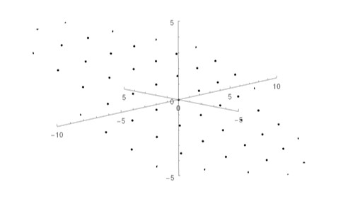
Eventually, we might want these "basis" vectors to be at right angles to facilitate applying textures and moving the object through space. This is possible using the Gram-Schmidt process, which we will learn about in Lecture 40.
« Lecture 9 Back to Top Lecture 11 »