In Lecture 10, we learned how to describe the solution set of a homogeneous matrix equation \( A \bbm x = \bbm 0 \). As we will see, the solution set of \( A \bbm x = \bbm b \), where \( \bbm b \neq \bbm 0 \), can be described in a similar way.
Example 1. Let \( A = \begin{bmatrix} 3 & 5 & -4 \\ =3 & -2 & 4 \\ 6 & 1 & -8 \end{bmatrix} \) and \( \bbm b = \vecthree 7 {-1} 4 \). Write the solution sets of \( A\bbm x = \bbm 0 \) and \( A \bbm x = \bbm b \) in parametric vector form.
| Homogeneous | Non-Homogeneous | |
|---|---|---|
| The augmented matrix is \( \begin{bmatrix} 3 & 5 & -4 & 0 \\ -3 & -2 & 4 & 0 \\ 6 & 1 & -8 & 0 \end{bmatrix} \) | The augmented matrix is \( \begin{bmatrix} 3 & 5 & -4 & 7 \\ -3 & -2 & 4 & -1 \\ 6 & 1 & -8 & 4 \end{bmatrix} \) | |
| The row-reduced matrix is \( \begin{bmatrix} 1 & 0 & -4/3 & 0 \\ 0 & 1 & 0 & 0 \\ 0 & 0 & 0 & 0 \end{bmatrix} \) | The row-reduced matrix is \( \begin{bmatrix} 1 & 0 & -4/3 & -1 \\ 0 & 1 & 0 & 2 \\ 0 & 0 & 0 & 0 \end{bmatrix} \) | |
| The general solution is \( x_1 = \frac 4 3 x_3 \), \( x_2 = 0 \), and \( x_3 \) is free | The general solution is \( x_1 = \frac 4 3 x_3 - 1\), \( x_2 = 2 \), and \( x_3 \) is free | |
| The solution in parametric vector form is \( \vecthree {x_1} {x_2} {x_3} = x_3 \vecthree {4/3} 0 1 \) | The solution in parametric vector form is \( \vecthree {x_1} {x_2} {x_3} = x_3 \vecthree {4/3} 0 1 + \vecthree {-1} 2 0. \Box \) |
If we graph these two solution sets, we see that they represent two parallel lines in \( \mathbb R^3 \):
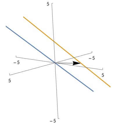
The blue line in the figure above passes through the origin, and represents the solution of \( A \bbm x = \bbm 0\). The orange line represents the solution of \( A \bbm x = \bbm b \). The arrow pointing from the blue line to the orange line is \( \bbm p = \vecthree {-1} 2 0 \), one of the many solutions of \( A\bbm x = \bbm b\).
In fact, every solution of \( A \bbm x = \bbm b \) can be written as \( \bbm v + \bbm p \), where \( \bbm v \) is any solution of \( A \bbm x = \bbm 0\) and \( \bbm p \) is any particular solution of \(A\bbm x = \bbm b\). This means that we can construct the solution set of \( A \bbm x = \bbm b \) using two "building blocks":
This way of describing the solutions of \( A \bbm x = \bbm b \) is a characterization. This is different from the definition of "solution." We know that a vector \( \bbm u \) being a solution of \( A \bbm x = \bbm b \) simply means that \( A \bbm u = \bbm b \). The characterization is equivalent to the definition (as we will prove) and provides a different way of looking at the meaning of the definition.
Theorem (Characterization of Solutions of Non-Homogeneous Equations). Let \( A \) be an \( m \times n\) matrix, let \( \bbm b \in \mathbb R^m \), and let \( \bbm p \) be any solution of \( A \bbm x = \bbm b \). The solution set of \( A \bbm x = \bbm b\) is the set of all vectors of the form \( \bbm v + \bbm p \), where \( \bbm v \) is a solution of \( A \bbm x = \bbm 0\).
To prove this theorem, we have to show that two sets are equal: (1) the solution set of \( A \bbm x = \bbm b\) and (2) the set of vectors of the form \( \bbm v + \bbm p \). To do this, we will have to show that any vector in set (1) is in set (2), and vice versa.
Proof, Part I. Let \( \bbm u \) be a solution of \( A \bbm x = \bbm b \). By defintion, this means that \( A \bbm u = \bbm b\). Now, \( \bbm u = (\bbm u - \bbm p) + \bbm p\). To show that \( \bbm u - \bbm p \) is a solution of \( A \bbm x = \bbm 0 \), we multiply: \[ A (\bbm u - \bbm p) = A\bbm u - A\bbm p = \bbm b - \bbm b = \bbm 0. \] Thus, we have shown that \( \bbm u \) has the form \( \bbm v + \bbm p \), where \( \bbm v = \bbm u - \bbm p \) is a solution of \( A \bbm x = \bbm 0 \).
Proof, Part II. Let \( \bbm u = \bbm v + \bbm p \), where \( \bbm v \) is a solution of \( A \bbm x = \bbm 0 \). To show that \( \bbm u \) is a solution of \( A \bbm x = \bbm b \), we multiply: \[ A \bbm u = A (\bbm v + \bbm p) = A\bbm v + A\bbm p = \bbm 0 + \bbm b = \bbm b. \] Thus, we have shown that \( \bbm u = \bbm v + \bbm p \) is a solution of \( A\bbm x = \bbm b . \Box \)
The characterization theorem tells us that, if we know all the solution of \( A\bbm x = \bbm 0\), then all we need is one solution of \(A\bbm x = \bbm b\) to figure out all solutions of \( A \bbm x = \bbm b\).
It is important to note that it is possible for \( A \bbm x = \bbm b \) to have no solutions, even though \( A \bbm x = \bbm 0 \) always has at least one solution. In this case, the theorem does not apply, since there is no vector \( \bbm p \) that we can use as a "building block."
The characterization theorem is an example of a statement about vectors and solutions of equations. In general, we will want to be able to prove statements of the form "If vector \( \bbm u \) has Property X, then vector \( \bbm v \) has Property Y." For these types of proofs, follow this outline:
Example 2. Let \( A \) be an \( m \times n \) matrix and let \(\bbm w \in \mathbb R^n \). Prove that if \( \bbm w \) is a solution of \( A \bbm x = \bbm 0\), then every scalar multiple of \( \bbm w \) is a solution of \( A \bbm x = \bbm 0 \).
We start by writing "Let \( \bbm w \in \mathbb R^n \) be a solution of \( A \bbm x = \bbm 0 \)." What does this tell us about \( \bbm w \)? Thinking about the definition of "solution," we might recall that this means that \( A \bbm w = \bbm 0 \).
Our goal is to show that "every scalar multiple of \( \bbm w \) is a solution of \( A \bbm x = \bbm 0 \)." We don't want to work with a specific scalar multiple like \( 3 \bbm w \), because this wouldn't show anything about any other scalar multiple. Instead, we work with a generic scalar multiple. We write "let \( c\ \bbm w \) be a scalar multiple of \( \bbm w\), for some scalar \( c \)."
How can we show that \( c\ \bbm w \) is a solution of \( A \bbm x = \bbm 0\)? We can use the defintion of solution again, this time by plugging \( c\ \bbm w\) in for \(\bbm x \) on the left-hand side and trying to see if we can show that this equals \( \bbm 0 \): \[ A(c \ \bbm w) = c(A\bbm w) = c(\bbm 0) = \bbm 0. \] This shows that, just like we wanted, \( c\ \bbm w \) is a solution of \( A \bbm x = \bbm 0. \Box \)
Here is a "clean" solution for Example 2, without the explanation and thought process:
Let \( \bbm w \in \mathbb R^n \) be a solution of \( A \bbm x = \bbm 0 \). By definition, \( A \bbm w = \bbm 0 \). Let \( c\ \bbm w \) be a scalar multiple of \( \bbm w\), for some scalar \( c \). Now, \( A(c \ \bbm w) = c(A\bbm w) = c(\bbm 0) = \bbm 0 \), so \( c\ \bbm w \) is a solution of \( A \bbm x = \bbm 0. \Box \)
« Lecture 10 Back to Top Lecture 12 »