Economies are complex, consisting of countless companies and consumers. Economists often model economies using sectors, each of which outputs goods and/or services that are then purchased or consumed by other sectors. Over time, economic theory states that these systems will settle into equilibrium, where the income of each sector exactly balances its expenses.
To illustrate how this works, and how our linear algebra ideas apply, we will work with a simple example involving three sectors: Transportation, Electricity, and Manufacturing. We can model the exchange of goods and services between these sectors visually:
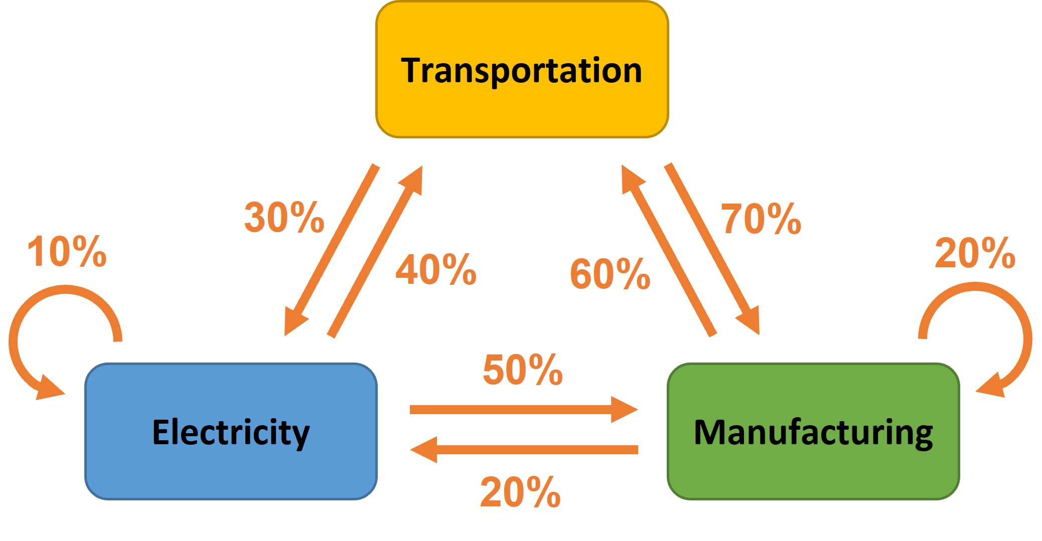
To read this diagram, follow the arrows out of each sector to see how that sector's output is sold. For example, the output from the Manufacturing sector is divided like this:
We can also model the inputs and outputs with a table:
| Distribution of output from... | |||
| Transp. | Elec. | Manuf. | purchased by... |
| 0% | 40% | 60% | Transportation |
| 30% | 10% | 20% | Electricity |
| 70% | 50% | 20% | Manufacturing |
In this table, each column shows the distribution of the output from that sector. So, each column must add up to 100%, but the rows need not add up to 100%.
At any given moment, the state of the economic model may not be in equilibrium. We can "transition" from one state to the next by applying the percentages in the model.
Example 1. Suppose that the values of each sector in the input-output model above are:
What are the values in the next state?
We can represent this economic state with a vector \( \vecthree {p_T} {p_E} {p_M} = \vecthree {100} {50} {200} \). The "\( p \)" variables represent the value, or "price" of each sector. This is the amount of money that would need to be paid to purchase 100% of that sector.
To find the prices in the next state, we apply the percentages. We assume that all of the output from a sector gets purchased (including possibly partially by the sector itself) since a sector will not want to wastefully produce more than it can sell. Looking at Transportation, we see that this sector purchases 40% of Electricity (for \( 0.4 \cdot 50 = \) $20 million) and 60% of Manufacturing (for \( 0.6 \cdot 200 = \) $120 million). This tells us that, in the next state, the price of Transportation will be \( 20 + 120 = \) $140 million.
In fact, the next states can be computed by multiplying our state vector by the matrix represented by the table: \[ \begin{bmatrix} 0 & 0.4 & 0.6 \\ 0.3 & 0.1 & 0.2 \\ 0.7 & 0.5 & 0.2 \end{bmatrix} \vecthree {100} {50} {200} = \vecthree {140} {75} {135} \]
Write \( M \) be the matrix represented by the input-output table. We call \( M \) a "transition" matrix because multiplying by \( M \) "transitions" us from one state to the next. We can see that \( \vecthree {100} {50} {200} \) does not represent the equilibrium, since \( M \vecthree {100} {50} {200} \neq \vecthree {100} {50} {200} \).
We can multiply by \( M \) again to get: \[ M \vecthree {140} {75} {135} = \begin{bmatrix} 0 & 0.4 & 0.6 \\ 0.3 & 0.1 & 0.2 \\ 0.7 & 0.5 & 0.2 \end{bmatrix} \vecthree {140} {75} {135} = \vecthree {111} {76.5} {162.5}. \]
Repeatedly multiplying by the transition matrix will eventually lead us closer and closer to the equilibrium we are seeking.
To find the equilibrium prices more efficiently, we must realize that we are looking for a vector \( \bbm x \) for which \( M \bbm x = \bbm x\). This is a matrix equation that looks different from the ones we have studied so far, but we can still apply our techniques to find \( \bbm x \) directly.
Let \( \bbm x = \vecthree {p_T} {p_E} {p_M} \). Writing \( M \bbm x = \bbm x \) as a system of equations gives \[ \begin{eqnarray*} 0.4 p_E + 0.6 p_M & = & p_T \\ 0.3 p_T + 0.1 p_E + 0.2 p_M & = & p_E \\ 0.7 p_T + 0.5 p_E + 0.2 p_M & = & p_M \end{eqnarray*} \]
Now we move the variables to the left-hand side: \[ \begin{eqnarray*} -1p_T + 0.4 p_E + 0.6 p_M & = & 0 \\ 0.3 p_T - 0.9 p_E + 0.2 p_M & = & 0 \\ 0.7 p_T + 0.5 p_E - 0.8 p_M & = & 0 \end{eqnarray*} \]
Next, we set up and row-reduce the corresponding augmented matrix: \[ \begin{bmatrix} -1 & 0.4 & 0.6 & 0 \\ 0.3 & -0.9 & 0.2 & 0 \\ 0.7 & 0.5 & -0.8 & 0 \end{bmatrix} \longrightarrow \begin{bmatrix} 1 & 0 & -0.795 & 0 \\ 0 & 1 & -0.487 & 0 \\ 0 & 0 & 0 & 0 \end{bmatrix}. \]
This gives us our solution in parametric vector form: \[ \vecthree {p_T} {p_E} {p_M} \approx p_M \vecthree {0.795} {0.487} 1. \]At this point, we see that there are infinitely many solutions. If we had an additional piece of information, we can use that to find a specific set of equilibrium prices.
Example 2. Suppose that, in the input-output model above, the price of Manufacturing at equilibrium is $100 million. What are the other equilibrium prices?
Since \( p_M = \) $100 million, we compute \( \vecthree {p_T} {p_E} {p_M} \approx 100 \vecthree {0.795} {0.487} 1 = \vecthree {79.5} {48.7} {100}\). So, the equilibrium price of Transportation is $79.5 million and the equilibrium price of Electricity is $48.7 million. \( \Box \)
Example 3. Suppose that the total price of the economy in the input-output model above is $300 million. What are the equilibrium prices?
This time, we don't know what \( p_M \) is, but we do know that \( p_T + p_E + p_M = 300\). Substituting, we have \( 0.795 p_M + 0.487 p_M + p_M = 300 \), or \( 2.282 p_M = 300 \). Solving for \( p_M \), we get \( p_M = \) $131.5 million. We can then find \( p_T = \) $104.5 million and \( p_E = \) $64.0 million.
Input-output models are an example of a Markov chain. In a Markov chain, we have a transition matrix \( M \) where we repeatedly multiply by \( M\) and try to find an equilibrium state where \( M \bbm x = \bbm x\). In Lecture 33, we will study equations of this nature and begin to learn ways to better model repeatedly multiplying a vector by the same matrix.
« Lecture 11 Back to Top Lecture 13 »