
When defining a function, we often write \( f : X \to Y \), where \( f \) is the name of the function, \( X \) is the domain (the set of possible inputs for \( f\) ), and \( Y \) is the codomain (the set of possible outputs for \( f\)).
Definition. Given an \( m\times n \) matrix \( A \), we can define the matrix transformation corresponding to \( A \), which is the function \( T : \mathbb R^n \to \mathbb R^m \) defined by the rule \( T(\bbm x) = A \bbm x \).
With the above notation, the domain of \( T \) is \( \mathbb R^n \), where \( n \) is the number of columns of \( A \), and the codomain of \( T \) is \( \mathbb R^m \), where \( m \) is the number of rows of \( A \).
Example 1. Let \( A = \begin{bmatrix} 2 & 0 & -3 \\ -1 & 4 & 5 \end{bmatrix} \) and let \( T : \mathbb R^3 \to \mathbb R^2 \) be defined by \( T(\bbm x) = A\bbm x \). Evaluate \( T \left( \vecthree 1 2 3 \right) \).
We compute \[ T \left( \vecthree 1 2 3 \right) = A \vecthree 1 2 3 = \begin{bmatrix} 2 & 0 & -3 \\ -1 & 4 & 5 \end{bmatrix} \vecthree 1 2 3 = \vectwo {-7} {22}.\ \Box \]
Any function \( T : \mathbb R^n \to \mathbb R^m \) is called a transformation, so matrix transformations are just a specific type of transformation.
Definitions. Given a transformation \( T : \mathbb R^n \to \mathbb R^m \) and a vector \( \bbm x \in \mathbb R^n \), the vector \( T(\bbm x) \) is the image of \( \bbm x \) under \( T \). The subset of \( \mathbb R^m \) containing all images of \( T \) is called the range (or image) of \( T \).
Note that, depending on \( T \), the range of \( T \) might be all of \( \mathbb R^m \), meaning that every vector in \( \mathbb R^m \) is an image of \( T \). We will consider this possibility in detail in Lecture 20.
Example 2. Let \( A = \begin{bmatrix} 1 & -3 \\ 3 & 5 \\ -1 & 7 \end{bmatrix} \) and define \( T : \mathbb R^2 \to \mathbb R^3 \) by \( T(\bbm x)=A\bbm x\).
For part (a), we compute \( T \left( \vectwo 2 {-1} \right) = A \vectwo 2 {-1} = \vecthree 5 1 {-9} \).
For part (b), we must solve the equation \( T(\bbm x) = \vecthree 3 2 {-5} \), which is the same as the equation \( A\bbm x = \vecthree 3 2 {-5}\). We set up and row-reduce an augmented matrix for this matrix equation: \[ \begin{bmatrix} 1 & -3 & 3 \\ 3 & 5 & 2 \\ -1 & 7 & -5 \end{bmatrix} \longrightarrow \begin{bmatrix} 1 & 0 & 3/2 \\ 0 & 1 & -1/2 \\ 0 & 0 & 0 \end{bmatrix} \] The solution is \( \bbm x = \vectwo {3/2} {-1/2} \).
For part (c), we are asked whether it is possible to write \( \bbm c = T(\bbm x) \) for some vector \( \bbm x \in \mathbb R^2 \). We solve the equation \( T(\bbm x) = \bbm c \), which is equivalent to the matrix equation \( A \bbm x = \vecthree 325\). Again, we row-reduce an augmented matrix: \[ \begin{bmatrix} 1 & -3 & 3 \\ 3 & 5 & 2 \\ -1 & 7 & 5 \end{bmatrix} \longrightarrow \begin{bmatrix} 1 & 0 & 0 \\ 0 & 1 & 0 \\ 0 & 0 & 1 \end{bmatrix} \] Since this augmented matrix has a pivot in the last column, the corresponding matrix equation has no solutions. This means that, no, \( \bbm c \) is not in the range of \( T \). \( \Box \)
Some matrix transformations can be visualized as operations in \( \mathbb R^2 \) or \( \mathbb R^3 \).
For example, consider the tranformation \( T(\bbm x) = A\bbm x \), where \( A = \begin{bmatrix} 1 & 0 & 0 \\ 0 & 1 & 0 \\ 0 & 0 & 0 \end{bmatrix} \). We have \( T \left( \vecthree x y z \right) = \vecthree x y 0 \). We can visualize this as a projection from three to two dimensions:
Here we see a three-dimensional sphere and its image under the transformation \( T \). This creates a two-dimensional "shadow" of the sphere in the \( xy \)-plane.
As another example, consider \( T(\bbm x) = A\bbm x \), where \( A = \begin{bmatrix} 1 & m \\ 0 & 1 \end{bmatrix} \). This is a "horizontal shear" transformation:

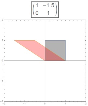
In the above images, we see the effect of two different horizontal shear transformations on a square (pictured in gray). The pink parallelogram shows the image of the square.
The transformation \( T(\bbm x) = A\bbm x \), where \( A = \begin{bmatrix} 1 & 0 \\ 0 & 1 \end{bmatrix} \), is called the identity transformation. For this transformation, \( T(\bbm x) = \bbm x \) for all vectors \( \bbm x \).
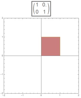
Here we see the gray square and its pink image, which perfectly overlap because they are the same square. While such a transformation may seem "boring," identity transformations play an important role in our study of matrix multiplication, starting in Lecture 21.
« Lecture 16 Back to Top Lecture 18 »