Definition. The standard basis vector (also called the elementary basis vector) \( \bbm e_j \) in \( \mathbb R^n \) has 1 in its \( j^{\rm th} \) entry and 0 in all other entries.
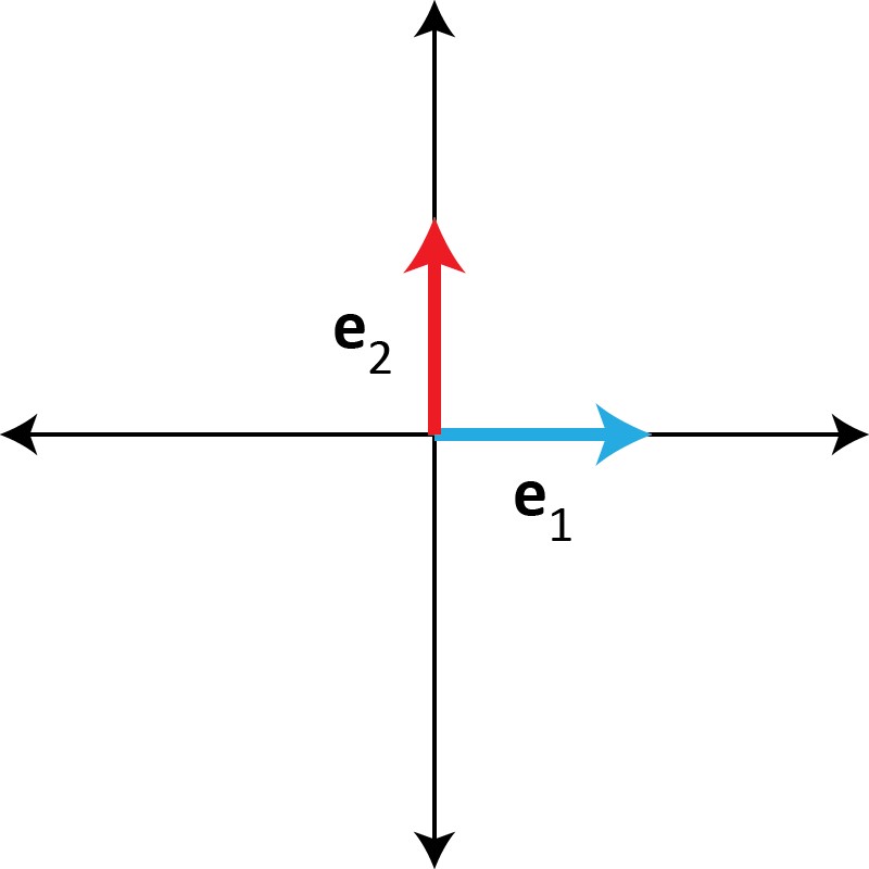
For example, in \( \mathbb R^2 \), the standard basis vectors are \( \bbm e_1 = \vectwo 10\) and \( \bbm e_2 = \vectwo 01 \).
In \( \mathbb R^3 \), the standard basis vectors are \( \bbm e_1 = \vecthree 100 \), \(\bbm e_2 = \vecthree 010 \), and \( \bbm e_3 = \vecthree 001 \). Note that this can cause some confusion since the notation "\( \bbm e_1 \)" can have different meanings depending on the context.
Given a linear transformation \( T : \mathbb R^n \to \mathbb R^m \), knowing the values \( T(\bbm e_j) \) for each \( j \) allows us to compute the value of \( T \) at any other vector in \( \mathbb R^n \). This is illustrated in the following example.
Example 1. Suppose that \( T : \mathbb R^2 \to \mathbb R^3 \) is a linear transformation where \( T\left( \vectwo 10 \right) = \vecthree 4 {-1} 2 \) and \( T\left( \vectwo 01 \right) = \vecthree 0 2 3 \). Compute \( T\left( \vectwo {3} {-5} \right) \).
We write \( \vectwo {3} {-5} = (3)\vectwo 10 + (-5) \vectwo 01 \) and use the linearity of \( T \): \[ T\left( \vectwo {3} {-5} \right) = T\left( 3\vectwo 10 + (-5) \vectwo 01 \right) = 3 T\left( \vectwo 10 \right) + (-5) T\left( \vectwo 01 \right) = 3 \vecthree 4 {-1} 2 + (-5) \vecthree 0 2 3 = \vecthree {12} {-13} {-9}. \ \Box \]
When \( T \) is a matrix transformation \( T(\bbm x) = A\bbm x \), finding the values \( T(\bbm e_j) \) is easy. Since \( \bbm e_j \) has 1 in its \( j^{\rm th} \) entry and 0 in all other entries, \( T(\bbm e_j) = A\bbm e_j \) is just the \( j^{\rm th} \) column of \( A\).
Example 2. Let \( T \) be the transformation \( T(\bbm x) = A\bbm x \), where \( A = \begin{bmatrix} 0 & -1 & 3 & 0 \\ 2 & 4 & -5 & 1 \\ 1 & 3 & 0 & -6 \end{bmatrix} \). Compute \( T(\bbm e_2 )\).
We compute \[ T(\bbm e_2 ) = A\bbm e_2 = \begin{bmatrix} 0 & -1 & 3 & 0 \\ 2 & 4 & -5 & 1 \\ 1 & 3 & 0 & -6 \end{bmatrix} \vecfour 0100 = 0 \vecthree 021 + 1 \vecthree {-1} 43 + 0 \vecthree 3 {-5} 0 + 0 \vecthree 01{-6} = \vecthree {-1} 4 3. \ \Box \]
In the previous lecture, we saw that every matrix transformation is a linear transformation and asked the question of whether there existed linear transformations that were not matrix transformations. The next theorem tells us that the answer to this question is "no."
Theorem (The Matrix of a Linear Transformation). Let \( T : \mathbb R^n \to \mathbb R^m \) be a linear transformation. Then, \( T \) is a matrix transformation \( T(\bbm x) = A\bbm x \), where \( A \) is the matrix whose \( j^{\rm th} \) column is \( T(\bbm e_j) \): \[ A = \begin{bmatrix} T(\bbm e_1) & T(\bbm e_2) & \cdots & T(\bbm e_n) \end{bmatrix} \]
Proof. Let \( \bbm x \in \mathbb R^n \) and write \( \bbm x = \vecfour {x_1} {x_2} \vdots {x_n} \). Then, we can rewrite \( \bbm x = x_1 \bbm e_1 + x_2 \bbm e_2 + \cdots + x_n \bbm e_n. \)
Using the linearity properties of \( T \), we have \( T(\bbm x) = T(x_1 \bbm e_1 + x_2 \bbm e_2 + \cdots + x_n \bbm e_n) = x_1 T(\bbm e_1) + x_2 T(\bbm e_2) + \cdots x_n T(\bbm e_n) \). Also, by the definition of matrix-vector multiplication, \[ A \bbm x = \begin{bmatrix} T(\bbm e_1) & T(\bbm e_2) & \cdots & T(\bbm e_n) \end{bmatrix} \vecfour {x_1} {x_2} \vdots {x_n} = x_1 T(\bbm e_1) + x_2 T(\bbm e_2) + \cdots x_n T(\bbm e_n) \]
This proves that \( T(\bbm x) = A\bbm x \). \( \Box \)
Definition. Given a linear transformation \( T\), the matrix \( A = \begin{bmatrix} T(\bbm e_1) & T(\bbm e_2) & \cdots & T(\bbm e_n) \end{bmatrix} \) is the standard matrix for \( T \).
We can use the theorem in this lecture to find the matrix of a linear transformation as long as we know what the transformation does to the standard basis vectors.
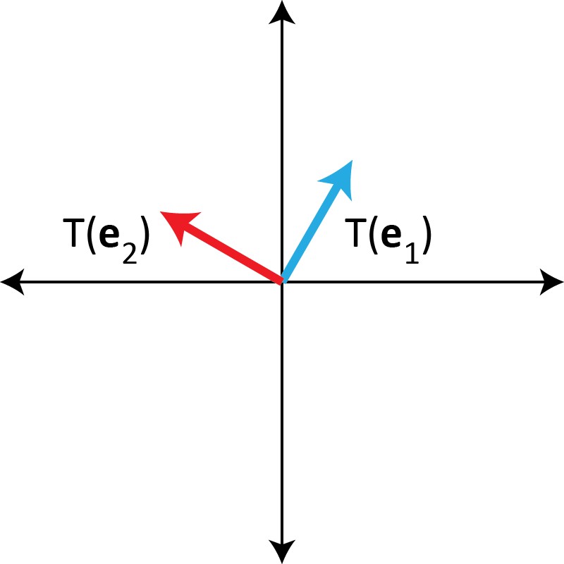
Example 3. Let \( T : \mathbb R^2 \to \mathbb R^2 \) be the transformation that represents a 60-degree counterclockwise rotation about the origin. Find the standard matrix for \( T\).
We can use trigonometry to compute \( T(\bbm e_1) \) and \( T(\bbm e_2) \).
We see that \( T(\bbm e_1) = \vectwo {1/2} {\sqrt 3/2} \) and \( T(\bbm e_2) = \vectwo {-\sqrt 3/2}{1/2} \), so the standard matrix for \( T \) is \( \begin{bmatrix} 1/2 & -\sqrt 3/2 \\ \sqrt 3/2 & 1/2 \end{bmatrix} \). \( \Box \)
We can also use limited information about \( T \) to reason about the columns of its standard matrix.
Example 4. Suppose that \( T : \mathbb R^3 \to \mathbb R^2 \) is a linear transformation where \( T \left( \vecthree 10{-1} \right) \) equals the zero vector. Explain why the first and third columns of the standard matrix for \( T \) are equal.
The key to this problem is to notice that \( \vecthree 10{-1} = \vecthree 100 - \vecthree 001 = \bbm e_1 - \bbm e_3 \). We are given that \( T(\bbm e_1 - \bbm e_3) = \bbm 0 \). Using the linearity of \( T \), we have \( T(\bbm e_1) - T(\bbm e_3) = \bbm 0 \), so \( T(\bbm e_1) = T(\bbm e_3) \). Since \( T(\bbm e_1)\) and \(T(\bbm e_3)\) are, respectively, the first and third columns of the standard matrix for \( T \), this explains why those two columns must be equal. \( \Box \)
Example 5. Suppose that \( T \) is a linear transformation where \( T \left( \vecthree {-2} {-1} 2 \right) = \vectwo {-5} 2 \) and \( T \left( \vecthree 1 1 {-1} \right) = \vectwo 3 7 \). Find the second column of the standard matrix for \( T \).
The question is asking us to compute \( T(\bbm e_2) \), so we need to be able to write \( \bbm e_2 \) as a linear combination of \( \vecthree {-2} {-1} 2 \)and \( \vecthree 1 1 {-1} \) so that we can apply the linearity of \( T \). We solve the vector equation \( x_1 \vecthree {-2} {-1} 2 + x_2 \vecthree 1 1 {-1} = \vecthree 010 \): \[ \begin{bmatrix} -2 & 1 & 0 \\ -1 & 1 & 1 \\ 2 & -1 & 0 \end{bmatrix} \longrightarrow \begin{bmatrix} 1 & 0 & 1 \\ 0 & 1 & 2 \\ 0 & 0 & 0 \end{bmatrix} \]
This tells us that the solution to the vector equation is \( x_1 = 1 \) and \( x_2 = 2 \), and so \( 1 \vecthree {-2} {-1} 2 + 2 \vecthree 1 1 {-1} = \vecthree 010 \). Now, the second column of the standard matrix for \( T \) is \[ T(\bbm e_2) = T\left( 1 \vecthree {-2} {-1} 2 + 2 \vecthree 1 1 {-1} \right) = 1 T \left( \vecthree {-2} {-1} 2 \right) + 2 T \left( \vecthree 1 1 {-1} \right) = 1 \vectwo {-5} 2 + 2 \vectwo 3 7 = \vectwo 1 {16}. \ \Box \]
« Lecture 18 Back to Top Lecture 20 »