Definition. A set of vectors \( \{ \bbm v_1, \bbm v_2, \ldots, \bbm v_p \} \) in \( \mathbb R^n \) is an orthogonal set if \( \bbm v_i \cdot \bbm v_j = 0 \) for all \( i \neq j \).
In an orthogonal set, every vector is orthogonal to every other vector. For example, the standard basis vectors \( \{ \bbm e_1, \bbm e_2, \ldots, \bbm e_n \} \) are mutually orthogonal, so they form an orthogonal set.
Example 1. Show that the set \( \bbm u_1, \bbm u_2, \bbm u_3 \) is orthogonal, where \( \bbm u_1 = \vecthree 311 \), \( \bbm u_2 = \vecthree {-1} 2 1 \), and \( \bbm u_3 = \vecthree {-1/2} {-2} {7/2} \).
We compute: \[ \bbm u_1 \cdot \bbm u_2 = (3)(-1) + (1)(2) + (1)(1) = 0 \] \[ \bbm u_1 \cdot \bbm u_3 = (3)(-1/2) + (1)(-2) + (1)(7/2) = 0 \] \[ \bbm u_2 \cdot \bbm u_3 = (-1)(-1/2) + (2)(-2) + (1)(7/2) = 0.\ \Box \]
Theorem (Orthogonal Sets Are Linearly Independent). If \( \{ \bbm v_1, \ldots, \bbm v_p \} \) is an orthogonal set of nonzero vectors, then this set is linearly independent.
Proof. Let \( \{ \bbm v_1, \ldots, \bbm v_p \} \) be an orthogonal set of nonzero vectors. Suppose \( c_1 \bbm v_1 + \cdots + c_p \bbm v_p = \bbm 0 \) for some scalars \( c_1, \ldots, c_p \). Our goal is to show that the \( c_i \) are all zero.
Take the dot product of \( \bbm v_i \) with both sides of this equation: \[ \bbm v_i \cdot (c_1 \bbm v_1 + \cdots + c_p \bbm v_p) = \bbm v_i \cdot \bbm 0 \] \[ c_1 (\bbm v_i \cdot \bbm v_1) + \cdots + c_i(\bbm v_i\cdot \bbm v_i) + \cdots + c_p (\bbm v_i \cdot \bbm v_p) = 0. \]
This equation simplifies to \( c_i(\bbm v_i \cdot \bbm v_i) = 0\) since the set is orthogonal. Now, \( \bbm v_i \cdot \bbm v_i = \| \bbm v_i \|^2 \), which is not zero since \( \bbm v_i \) is a nonzero vector. Thus, we must have \( c_i = 0 \). \( \Box \)
Definition. Let \( H \subseteq \mathbb R^n \) be a subspace. An orthogonal basis for \( H \) is a basis that is also an orthogonal set.
An orthogonal basis \( \cal B \) is useful because for any vector \( \bbm y\in H \) it is relatively easy to compute the coordinates \( [\bbm y]_{\cal B} \).
Theorem (Coordinates in an Orthogonal Basis). Let \( H \subseteq \mathbb R^n \) be a subspace and let \( {\cal B} = \{ \bbm v_1, \ldots, \bbm v_p \} \) be an orthogonal basis for \( H \). Let \( \bbm y\in H \) and write \( [\bbm y]_{\cal B} = \vecthree {c_1} \vdots {c_p} \). Then \( c_i = \frac {\bbm y \cdot \bbm v_i}{\bbm v_i \cdot \bbm v_i} \) for each \( 1 \le i \le p \).
Proof. By definition, we have \( \bbm y = c_1 \bbm v_1 + \cdots + c_p \bbm v_p \). Take the dot product of \( \bbm v_i \) with both sides: \[ \bbm y \cdot \bbm v_i = (c_1 \bbm v_1 + \cdots + c_p \bbm v_p) \cdot \bbm v_i \] \[ \bbm y \cdot \bbm v_i = c_1 (\bbm v_1 \cdot \bbm v_i) + \cdots + c_i (\bbm v_i \cdot \bbm v_i) + \cdots + c_p (\bbm v_p \cdot \bbm v_i) \]
Since \( \cal B \) is orthogonal, this simplifies to \( \bbm y \cdot \bbm v_i = c_i (\bbm v_i \cdot \bbm v_i) \). Thus, \( c_i = \frac {\bbm y \cdot \bbm v_i}{\bbm v_i \cdot \bbm v_i} \), as desired. \( \Box \)
Example 2. Let \( \bbm v = \vecthree 203 \) and \( \bbm w = \vecthree {-6} 1 4 \), and write \( H = {\rm Span}\{ \bbm v, \bbm w \} \). Show that \( {\cal B} = \{ \bbm v, \bbm w \} \) is an orthogonal basis for \( H \). Compute \( [\bbm u]_{\cal B} \), where \( \bbm u = \vecthree {18} {-2} 1 \).
To show \( \cal B \) is orthogonal, we compute \( \bbm v \cdot \bbm w = (2)(-6)+(0)(1)+(3)(4) = 0\). For \( [\bbm u]_{\cal B} \), we compute \[ \frac{\bbm u \cdot \bbm v}{\bbm v \cdot \bbm v} = \frac{39}{13} = 3 \] \[ \frac{\bbm u \cdot \bbm w}{\bbm w \cdot \bbm w} = \frac{-106}{53} = -2 \]
Thus, \( [\bbm u]_{\cal B} = \vectwo 3 {-2} \). \( \Box \)
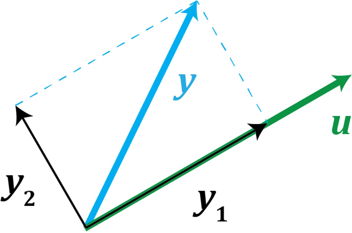
A common problem in physics and other fields of study is to decompose a vector into orthogonal components:
Given a vector \( \bbm u \in \mathbb R^n \), the general problem we want to solve is to decompose any vector \( \bbm y \in \mathbb R^n \) into a sum of two vectors \( \bbm y_1 + \bbm y_2 \), where \( \bbm y_1 \) is parallel to \( \bbm u \) and \( \bbm y_2 \) is orthogonal to \( \bbm u\). We say that \( \bbm y_1 \) is the "orthogonal projection" of \( \bbm y \) onto \( \bbm u\):
Definition. Let \( \bbm u, \bbm y \in \mathbb R^n \) be nonzero vectors. The orthogonal projection of \(\bbm y\) onto \( \bbm u \) is \( {\rm proj}_{\bbm u} \bbm y = \frac{\bbm y\cdot\bbm u}{\bbm u \cdot \bbm u} \bbm u\).
Theorem (Orthogonal Projection). Let \( \bbm u, \bbm y \in \mathbb R^n \). Write \( \bbm y_1 = \frac{\bbm y\cdot\bbm u}{\bbm u \cdot \bbm u} \bbm u\) and \( \bbm y_2 = \bbm y - \bbm y_1 \). Then
Proof. Statements (1) and (2) are clear from the definitions. For (3), we compute \[ \bbm y_2 \cdot \bbm u = \left( \bbm y - \frac{\bbm y\cdot\bbm u}{\bbm u \cdot \bbm u} \bbm u \right) \cdot \bbm u = \bbm y\cdot \bbm u - \frac{\bbm y\cdot\bbm u}{\bbm u \cdot \bbm u}(\bbm u \cdot \bbm u) = 0.\ \Box \]
Note the similarity between the orthogonal projection formula and the formula in the Coordinates in an Orthgonal Basis Theorem. Assuming \( \bbm u \) and \( \bbm y \) are not parallel, we can think of \( {\cal B} = \{ \bbm u, \bbm y_2 \} \) as an orthgonal basis for the subspace spanned by \( \bbm u \) and \( \bbm y \). The orthogonal projection \( \bbm y_1 \) is parallel to \( \bbm u \) and so \( \bbm y_1 = \alpha \bbm u \) for some scalar \( \alpha \). Clearly, \( [\bbm y_1]_{\cal B} = \vectwo \alpha 0 \), but by the Coordinates in an Orthogonal Basis Theorem we also have \( \alpha = \frac{\bbm y\cdot \bbm u}{\bbm u \cdot \bbm u} \).
Example 3. Let \( \bbm u = \vecthree 1 {-2} 4 \) and \( \bbm y = \vecthree 0 3 {-5} \). Compute \( {\rm proj}_{\bbm u} \bbm y \), the orthogonal projection of \( \bbm y \) onto \( \bbm u \).
We compute: \[ {\rm proj}_{\bbm u} \bbm y = \frac{\bbm y\cdot\bbm u}{\bbm u \cdot \bbm u} \bbm u = \frac{-26}{21} \bbm u = \vecthree {-26/21} {52/21} {-104/21}.\ \Box \]
Example 4. Let \( \bbm p = \vecfour {-1} 2 1 {-3} \) and \( \bbm q = \vecfour 0 {-4} 1 1 \). Decompose \( \bbm p = \bbm p_1 + \bbm p_2 \), where \( \bbm p_1 \) is parallel to \( \bbm q \) and \( \bbm p_2 \) is orthogonal to \( \bbm q \).
From our earlier discussion, we know \( \bbm p_1 = {\rm proj}_{\bbm q} \bbm p \) and \( \bbm p_2 = \bbm p - \bbm p_1 \). We compute: \[ \bbm p_1 = {\rm proj}_{\bbm q} \bbm p = \frac{\bbm p \cdot \bbm q}{\bbm q \cdot \bbm q} \bbm q = \frac{-10}{18} \bbm q = \vecfour 0 {20/9} {-5/9} {-5/9}. \] \[ \bbm p_2 = \bbm p - \bbm p_1 = \vecfour {-1} 2 1 {-3} - \vecfour 0 {20/9} {-5/9} {-5/9} = \vecfour {-1} {-2/9} {14/9} {-22/9}.\ \Box \]
« Lecture 37 Back to Top Lecture 39 »