Section 4: Derivatives

4.1 The Main Pillar of the Temple

In the last section we saw two examples of deriving a function from another function. In both cases we used the same recipe. The recipe is this:

If you have a function, f(x), and you want to find the value of the derived function at x, then find both f(x) and f of a nearby point, x + h, take the difference of those two values, and divide that by h. When you take the limit of that quotient (which is commonly called the divided difference) as h (which is the distance between x and the point that is nearby) goes toward zero, you have the derived function.

That is what we did to find the grade of the wall that the animals built. We knew the height of the wall at any point. Each animal used the divided difference (his change in altitude divided by his horizontal step size) to determine his own perception of the wall's grade. We used smaller and smaller animals to see what happens as their horizontal step size goes toward zero. And we saw that a limit exists. That limit was the derived function that gave us the exact grade at an exact point on the wall. We derived it from the function that gives us the height of the wall.

That is what we did also to determine instantaneous speed. We took the difference between where we are now and where we will be in a little while, and we divided that by the time elapsed over that little while. As the little while goes toward zero, we found that there was a limit, and that limit is the instantaneous speed. We derived the speed function from the function that gives us position as a function of time.

So here is the main idea: Take real function of a real variable, f(x). Form the divided difference of f(x):

    f(x + h) - f(x)
                                                                 eq. 4.1-1
           h

In other words, take the difference between what the function is at x and what it is a short distance, h, from x, then divide by the short distance, h. If you take the limit as h goes toward zero, and that limit exists, then you have the derived function's value at x. The derived function is called the derivative.

The concept of taking this limit of the divided difference to find the derivative is so commonly used in mathematics that we have special notations for it. If f(x) is a function and we find the limit of the divided difference exists over some domain, then we can express the derivative of f(x) as either f'(x) or as

   df
     
   dx

The first notation is due to Isaac Newton. You can see a brief biograpy of Isaac Newton by clicking here. The second is due to Gottfried Leibniz, who wanted to show that the derivative was a quotient of the differential in the function, f, divided by the differential in x. Leibniz imagined that the difference in both the numerator and in the denominator of 4.1-1 had an infinitesimal existence even as they both went to zero. He coined the term, differential, to describe such infinitesimal quantities. You can see a brief biography of Gottfried Leibniz by clicking here. Today both notations are in common use. Yet another notation you might see in some books would have a dot above the function name (which in this case is f) instead of the tick mark just to its right.

Important: The definition of the derivative of any function, f(x), is:

df f(x + h) - f(x) f'(x) = = lim eq. 4.1-2 dx h > 0 h

wherever that limit exists.

More on the "`d`" Notation

There really is nothing about Leibniz' "d" notation that is not contained in the limit equation given in equation 4.1-2. If we let the symbol, Dx, be the same as h, and if we let the symbol, Df, be the same as f(x + h) - f(x) (which is the same as f(x + Dx) - f(x) ), then equation 4.1-2 becomes

             df               Df
   f'(x)  =      =     lim                                        eq. 4.1-2a
             dx      Dx  > 0  Dx

So from a notation point of view, it's just another way of notating this limit of a ratio. The D operator stands for "difference." Dx is the difference between this x and another x a little ways away. Df is the difference between f of this x and f of the x that's a little ways away. The d operator stands for what happens to those differences in the limit. Which brings up an important point. The d and the D are both operators, NOT numbers. So when you see a d or a D in both numerator and denominator, you cannot cancel them. But if you saw a dx/dx, that you can cancel and say that it is equal to 1. That's because the dx in the numerator is identical to the dx in the denominator. Likewise if you saw Dx/Dx.

In Leibniz' way of looking at things, the symbol, dx, means that when you take the limit as Dx goes to zero, dx is the value that Dx takes on the instant before it winks out entirely and becomes zero. There is no real number that describes dx. It is closer to zero (though not equal to zero) than any nonzero real number can possibly be. Likewise df is the value that Df takes on the instant before Dx winks out entirely and becomes zero. Presumably Df winks out as well at that point, but remember that we are interested in the value of Df immediately before that happens. Again there is no real number that can describe df because it is closer to zero than any nonzero real number can possibly be. Yet although both dx and df are infinitesimal, their ratio is real whenever the limit exists. And that ratio, df/dx, is the derivative.

(For what it's worth to this discussion, mathematicians have devised an entirely self-consistent system of arithmetic among infinitesimal quantities. And yes, there is a whole tinier set of infinitessimal quantities that are as tiny compared to the infinitessimals we have been discussing as the ones we have been discussing are to the reals. They are the d² infinitessimals. And there is a set of even tinier infinitessimals for d³, and so on indefinitely)

When you think about it, the Leibniz notation better indicates what is going on when you take a derivative than does the Newton notation. For one thing, it clearly shows that a derivative of a function is taken with respect to a particular independent variable. In this case, that variable is x. It also shows that a derivative is always a ratio or quotient that happens in the limit as its denominator goes to zero (of course the numerator must go to zero at the same time for the limit to exist). Still the Newton notation is a convenient shorthand that requires fewer pencil strokes and fewer keystrokes at the keyboard. That is why I'll be using mostly the Newton notation throughout this tutorial.

The Derivative Is a Slope

You recall that in algebra you described straight lines that were not vertical using the equation, y = mx + b. And you recall as well that the term, m, you called the slope of the line. Suppose we take such a line as a function:

   f(x)  =  mx + b                                               eq. 4.1-3

If you make up values for m and b and plot it, you will find that it is indeed a straight line. Let's apply the definition given by 4.1-2 to find the derivative of this function.

                    (m(x + h) + b)  -  (mx + b)
   f'(x)  =   lim                                                eq. 4.1-4
             h  > 0              h

Do you see how we got 4.1-4 from 4.1-2 and 4.1-3? Make sure you understand how to make those substitutions. You are likely to have to do it on an exam.

When you multiply out the m(x + h), you get:

                    mx + mh + b  -  mx - b
   f'(x)  =   lim                                                eq. 4.1-5
             h  > 0           h

There are some major cancellation here. Once you do them, you are left with:

                    mh
   f'(x)  =   lim                                                eq. 4.1-6
             h  > 0  h

And when you apply the rule we discovered back in section 2.5, you get, simply

   f'(x)  =  m                                                   eq. 4.1-7

That means that the derivative of a straight line function (also called a linear function) is exactly its slope, m. And it doesn't matter what you choose for x. The derivative of a straight line is everywhere equal to its slope..

But what about functions that are not straight lines? What do their derivatives mean? Back in algebra, you talked about straight lines and their slopes. You also talked about parabolas and other curves, but you never talked about their slopes.

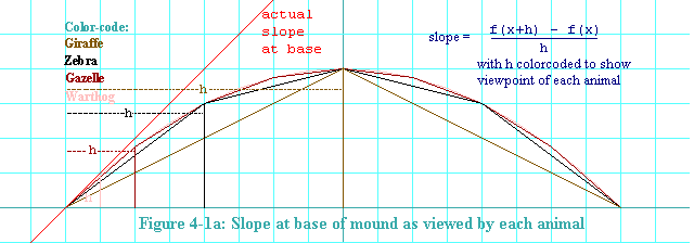
Remember the wall that the animals built? It was a parabola, wasn't it. The animals wanted to know its grade, but that is just a different word for slope. Here again is the diagram of the animal's pile of dirt as seen by the different animals. This time it shows the h each animal used to reckon the slope at the base of the mound. Starting at the base of the wall, each animal found a straight line that intersected the parabola at two points. Figure 4-1 Each animal determined the slope of that line and called that the grade at the base. We subsequently discovered that as you bring the two points of intersection closer and closer together, the slope of the resulting line approaches a limit. And at the limit, we have a line that is tangent to the wall. We are finding the slope of that tangent line, which is shown in red in the diagram.

That is how a derivative is a slope. If when you graph f(x) you get some curve, then the derivative, f'(x), gives you the slope of the line that is tangent to that same curve at x.

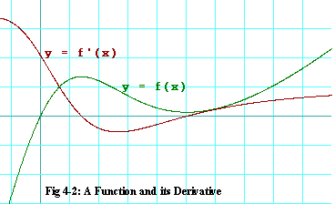
Figure 4-2 shows an arbitrary function graphed in green together with its derivative, which is graphed in brown. Fig. 4-2: A Function and its Derivative Never mind what the equation is for f(x). That is unimportant for now. Instead, look carefully at the behavior of the two functions. From x = -1 to x = 0, the green function increases by almost 3 squares. In that region it is sloping nearly 3 squares up for every square to the right. In that same region, the brown function, which is the derivative of the green function, is between +2 and +3. That is because the brown function graphs the slope of the green function.

From x = 0 to x = 1, the green function grows less steep. In other words, its slope lessens. At the same time, the brown function goes down, because it is representing the lesser slope of the green function.

Somewhere between x = 1 and x = 2 the green function levels out completely, that is, its slope becomes zero. At the corresponding x value, the brown function is zero.

From that point to about x = 5, the green function is sloping down, that is, it has a negative slope. In that entire region, the brown function is less than zero, as you would expect.

At about x = 5, the green function levels out again, having at that point a slope of zero. At that same x value, the brown function is again zero. To the right of that, the green function slopes back up again, and correspondingly the brown function is positive in that region.

You might try holding a straight edge up to the screen, tangent to the green function in various places. Count the squares up and squares to the right that the straight edge traverses, then use the quotient of squares up divided by squares to the right to estimate the slope of the green function at the point of tangency. Then compare your estimate to the value of the brown function at the same x.

The Derivative Is a Rate

Let's attach a different story to figure 4-2. Let's say that the horizontal axis measures seconds. For the green function, the vertical function measures tens of meters. In fact, it measures your progress down the road in your car. The story the green function tells goes something like this: "Prior to time -1 seconds, you were tooling along at about 30 meters per second (66 miles per hour) when you spotted a 50 dollar bill in the road. You screeched a halt, coming to a stop at about time 1.5 seconds. You immediately threw it into reverse, backed up, halted again, this time at about time 5 seconds, when you came even with the bill. Right away you snatched it up, then proceded on your way, but at a lesser speed." In this story, the brown graph shows exactly how fast you were going at each second in tens of meters per second. When you were going in reverse, your speed is considered negative. The brown graph is your rate.

In algebra you probably solved rate problems ad nauseum. But in all the problems, the rate (e.g. speed, dollars per hour, yen per Deutschmark, etc.) remained constant throughout the problem. Even when the rate did change, it changed in jumps (e.g. For 4 hours you are paid $5 per hour, then for the next four hours you are paid $8 per hour). The math you were learning then just wasn't up to dealing with rates that changed constantly with time. Yet the real world is full of rates that do change constantly with time or with other variables. And that is why you are learning calculus now. The concept of a derivative is simply a rate that can change constantly with time or with some other variable. It is the most central concept in calculus, even though the concept of limits underlies it. The derivative has some remarkable properties that you will learn about shortly. Those properties are so elegant that you will eventually come to know the derivative primarily by its properties, and that's how it should be. But don't ever forget that you came to the derivative by taking a limit. When you get confused, come back to that. Everthing you need to know about derivatives is hidden in the definition given here in equation 4.1-2.

Link to Important Coached Exercise

It is with near certainty that you will be required on some exam to find the derivative of some function by applying equation 4.1-2. So here I give you a coached exercise for finding the derivative of f(x) = x². In the same box we shall cover how you can find the derivative of g(x) = xⁿ where n is any counting number. So to dive deeply into derivatives, click here.

Return to Table of Contents

Move on to section 4.2: Rules to Live By